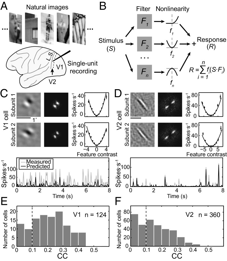
Fig. 1.
Analysis of RF subunits. (A) Random sequences of natural images were presented and single-unit recordings were made in either V1 or V2. L.S., lunate sulcus; dashed line, V1/V2 border. (B) Linear-nonlinear RF model. Each subunit is represented by a linear filter (Fi) depicting the spatial RF structure. S, stimulus. The response (xi = S·Fi) of each linear filter is passed through a second-order polynomial fi(xi) = ai + bixi + cixi2 before summation. n, number of subunits; i, the ith subunit; R, neuronal response. (C and D) Prediction of responses by RF models of example V1 (C) and V2 (D) cells. (Upper) Left, spatial RF; Center, spatial spectrum of RF; Right, static nonlinear function, with data points (mean ± SEM) depicting measured responses and curves representing polynomial fits of the data. (Lower) Gray, measured responses in test data set; black, model prediction. CC between measured (test data) and predicted responses was 0.38 in C and 0.37 in D. (E and F) Distribution of CCs for V1 and V2 cells. Black dashed line, threshold for all cells used for further RF analysis.

