Figure 4. Extracellular electrophysiology during whisker-guided locomotion.

(a) Schematic showing silicon probe recordings during open loop trials. The wall was moved in and out of different fixed distances from the mouse during a period of 4 s. (b) Coronal section through the brain of an Scnn1a-Tg3-Cre x RCL-ChR2-EYFP mouse acquired with green filter showing the barrels. Image acquired with orange filter is superimposed on top showing the track of the silicon probe coated in DiI. Electrolytic lesion is seen at the end of the DiI trace. Location of the probe is identified as C3 barrel. (c) Example spike rasters of regular spiking units during open-loop trials. Each row of the raster corresponds to one trial and each dot corresponds to one spike. The color of each dot represents the position of the wall at the time of the spike. Recordings are performed around C1 and C2 barrels. Only trials with running speed over 3 cm/s are represented. (d) Corresponding tuning curves to wall distance for the spike rasters shown in B (mean ± SE over trials). (e) Histogram of the location of tuning curve peaks. (f) Scatter plot of tuning curve suppression vs. activation. Activation is the difference between peak rate and baseline rate when the wall is out of reach. Suppression is the difference between minimum rate and baseline rate. (g) Heatmaps of z-scored tuning curves for units activated by more than 1 Hz (top) and units suppressed by more than 1 Hz (bottom) sorted by the location of the maximum and minimum wall distances respectively. Units that were both activated and suppressed appear in both plots. (h) Histogram of the tuning modulation, defined as the ratio of the difference between the activation and suppression divided by the sum of the activation and suppression. Units that are just activated have modulation 1, units that are just suppressed have modulation −1, and units that are both activated and suppressed have a modulation near 0. (i) Modulation index as a function of laminar position. Light gray, units classified as layer 2/3; medium gray, layer 4; dark gray, layer 5.

DOI: http://dx.doi.org/10.7554/eLife.12559.007

Figure 4—figure supplement 1. Electrophysiological methods.

(a) Image acquired with green filter of a whole brain removed from the skull of a Scnn1a-Tg3-Cre x RCL-ChR2-EYFP mouse. Overlay of 13 recordings sites identified by DiI tracing of silicon probe tracks. An image acquired with orange filter and superimposed on top for one example. The recording site is shown by arrow. (b) Illustration of three complementary methods used for identification of the depth of recorded units. Left: Coronal section of barrel cortex acquired with green and orange filters showing with dotted square the location of recording site. Center: Blown-up portion of the same area of the coronal section (turned rotated by 39 degrees) taken with green filter showing of L4 barrels. The location of two electrolytic lesions on top and bottom electrodes and the center of layer 4 are marked with dashed white lines. Right: Current source density trace used to identify the middle of Layer 4 as a short-time (<3 ms) minimum. The schematics of electrodes positions on the silicon probe that is aligned with the centers of the top and bottom lesions. (c) Inter-spike-interval distributions for units presented in Figure 4 and Figure 5. (d) Histogram of spike widths. Fast spikers (< 350 μs): pink, intermediate: gray, and regular spikers (> 450 μs): purple). (e) Z-scored waveforms from all units. (fast spikers: pink, intermediate: gray, regular spikers: purple). (f) Scatter plot of waveform SNR against ISI false alarm rate. The area shown by colored square corresponds to accepted units with SNR > 6 and false alarm rate < 1.5%

DOI: http://dx.doi.org/10.7554/eLife.12559.008

Figure 4—figure supplement 2. Lamina distribution of units.

(a) Distribution of the location of regular spiking units by depth relative to the middle of Layer 4. (b) Depth distribution of a baseline spike rate of regular spiking units during locomotion (speed over 3 cm/s). Light gray, units classified as layer 2/3; medium gray, layer 4; dark gray, layer 5. (c) Depth distribution of a peak spike rate of regular spiking units during locomotion (speed over 3cm/s). Light gray, units classified as layer 2/3; medium gray, layer 4; dark gray, layer 5.

DOI: http://dx.doi.org/10.7554/eLife.12559.009

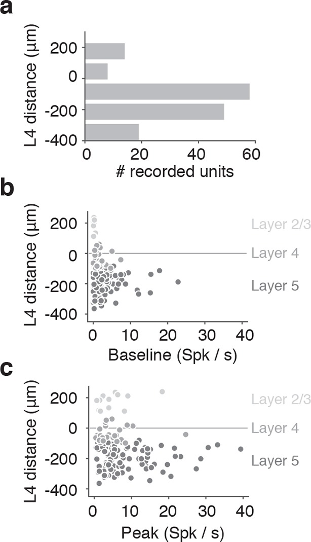
Figure 4—figure supplement 3. Comparison of open-loop and closed-loop tuning curves.

(a) Open-loop and closed-loop tuning curves for a regular spiking unit that gets activated by the wall. (b) Open-loop and closed-loop tuning curves for a unit that gets suppressed by the wall. (c) Scatter of the mean spiking rate of open-loop and closed-loop tuning curves. (d) Histogram of open vs. closed-loop modulation index which is the difference in open-loop and closed-loop spiking rates divided by the sum of open-loop and closed-loop spiking rates. Units that respond more during open loop trials have positive modulation, units that respond more during closed loop trials have negative modulation, and units that responded equally to both open and closed loop trials have a modulation of 0.

DOI: http://dx.doi.org/10.7554/eLife.12559.010

Figure 4—figure supplement 4. Effects of running speed on activity and wall distance tuning.

(a) Four example units that showed significant tuning to running speed when the wall was out of reach. The activity of the top left unit increased linearly with speed over a large range, the activity of top right unit increased rapidly and then saturated at low speeds, the activity of the bottom right unit peaked at low speeds and then decreased at higher speeds, and the activity of bottom left unit decreased with running speed. (b) Histogram of the peak speed tuning for units significantly tuned to speed (31%; 46/148) from the population used in Figure 4. (c) Example wall distance tuning curve while the mouse is running in fast trials (top) and slow trials (bottom). Fast and slow trials were split based on the median of the trial speeds in trials when the mouse was running. This unit is the same as used in Figure 4—figure supplement 3a). (d) Example wall distance tuning curve while the mouse is running fast trials (top) and slow trials (bottom). This unit is the same as used in Figure 4—figure supplement 3b). (e) Histogram of the modulation of wall distance tuning by speed for all 148 units. This index was the log of the gain parameter that describes a multiplicative scaling of the slow tuning curve to the fast tuning curve. Units that are more active during fast running have positive modulation indices, units that are less active during fast running have negative indices.

DOI: http://dx.doi.org/10.7554/eLife.12559.011

Figure 4—figure supplement 5. Tuning to ipsilateral and contralateral wall distance.

(a) Example spike raster of regular spiking unit in open-loop trials when the wall is contralateral (top) or ipsilateral to the recording site (bottom). Only epochs with running speed over 3 m/s are represented. This neuron was activated by interactions with the wall. (b) Corresponding tuning curves recorded during locomotion (running speed over 3 m/s). (c,d) Same as a, b for a suppressed regular spiking unit. (e) Scatter plot of range of spiking of ipsilateral vs. contralateral tuning curves. The range of spiking is the difference between the maximum and minimum of the tuning curve. (f) Histogram of laterality modulation index, which is the difference in contralateral range and ipsilateral range divided by the sum of the contralateral range and ipsilateral range. Units that respond only to the contralateral wall have modulation 1, units that respond only to the ipsilateral wall have modulation −1, and units that respond to both the contralateral and ipsilateral wall have a modulation near 0.

DOI: http://dx.doi.org/10.7554/eLife.12559.012