Figure 1. Schematic representation of the proposed pipeline.

(A) 3D multi-resolution image acquisition: example of arrays of 2D images of liver tissue acquired at different resolutions. Low- (1 μm × 1 μm × 1 μm per voxel) and high- (0.3 μm × 0.3 μm × 0.3 μm per voxel) resolution images on the left and right sides, respectively. (B) Multi-scale reconstruction of tissue architecture: on the left, reconstruction of a liver lobule showing tissue-level information, i.e., the localization and relative orientation of key structures such as the portal vein (PV) (orange) and central vein (CV) (light blue). The high-resolution images registered into the low-resolution one are shown in white. On the middle, a cellular-level reconstruction of liver showing the main components forming the tissue, i.e., bile canalicular (BC) network (green), sinusoidal network (magenta) and cells (random colours). The reconstruction corresponds to one of the high-resolution cubes (white) registered on the liver lobule reconstruction (left side). On the right, reconstruction of a single hepatocyte showing subcellular-level information, i.e., apical (green), basal (magenta) and lateral (grey) contacts. (C) Quantitative analysis of the tissue architecture: example of the statistical analysis performed over a morphometric tissue parameter (hepatocyte volume) using the information extracted from the multi-scale reconstruction. On the left, hepatocyte volume distribution over the sample (traditional statistics). On the right, spatial variability (spatial statistics) of the same parameter within the liver lobule. Our workflow allows not only to perform traditional statistical analysis of different morphometric parameters but also to perform spatial characterizations of them. The graphs were generated from the analysis of one high-resolution cube of the multi-scale reconstruction (the one shown in middle of panel B). Boundary cells were excluded from the analysis.

DOI: http://dx.doi.org/10.7554/eLife.11214.003

Figure 1—figure supplement 1. Workflow for the multi-scale reconstruction of tissue architecture from multi-resolution confocal microscopy images.

The necessary methods for each step (implemented in our software) are listed. They include newly developed ones (N) as well as standard image analysis algorithms (S) and modified versions of them (M).

DOI: http://dx.doi.org/10.7554/eLife.11214.004

Figure 1—figure supplement 2. Probabilistic image de-noising algorithm for 3D images.

Single 2D plane of a high-resolution image stained with phalloidin for actin (cell borders) and Flk1 for sinusoids (A, D) before and (B, E) after applying our probabilistic image de-noising algorithm. The outlier-tolerant estimation of the background was done using a 10-pixel window. (C, F) Phalloidin/Flk1 intensity values of pixels along the horizontal yellow line for both, the original and the de-noised images. Our probabilistic image de-noising algorithm efficiently reduces the noise while preserving the edges present in the image even in the presence of high diffusive background. (G) Mean variance for each intensity level (I). The experimental data are represented by the red dots, the error bar represents SEM and the theoretical curve (straight line) is represented by the solid black line. (H) Prediction of the background intensity using linear fitting by least-squares method (solid black line) and the outlier-tolerant algorithm (solid red line) for a set of sequential intensities in z-direction (blue dots). The dots represent the intensity values of the voxels along the vertical yellow line at the original image on the left [stained with CD13 for bile canalicular (BC) network].

DOI: http://dx.doi.org/10.7554/eLife.11214.005

Figure 1—figure supplement 3. Optimal parameter selection.

(A) The mask defining the objects vicinity in the case of bile canalicular (BC) network (yellow) is shown in red and was created by applying an inflation of two voxels (~0.5 µm) to the original objects. (B) Selection of the best parameters for the ‘pure denoise’ method. We used as fixed parameter the number of cycles (10, the maximum possible). ‘Number of frames’ = 11 (the maximum available in the plug-in) shows the best results, i.e., minimum global mean square error (MSE) as well as MSE in the vicinity of the objects. (C) Selection of the best parameters for the ‘edge preserving de-noising and smoothing’ method. We used as fixed parameter the number of cycles (100). ‘Smoothing level’ = 70 corresponds the point before the MSE in the vicinity of the objects starts increasing while the global MSE remains low.

DOI: http://dx.doi.org/10.7554/eLife.11214.006

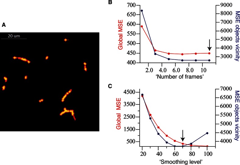
Figure 1—figure supplement 4. Comparison of our 3D image de-noising algorithm (BFBD) with standard methods in the field.

Panel (A) shows single 2D plane projections of an artificial high-resolution image of bile canalicular (BC) network (2:1 signal-to-noise ratio) before adding Poisson noise (ground truth) and the result of the application of our de-noising algorithm (BFBD) as well as a median filter, a Gauss low-pass filter and an anisotropic diffusion. (B) The resulting images were analysed in terms of the global mean square error (MSE) and coefficient of correlation (CoC). (C) The same metrics were evaluated only on the vicinity of the BC. Our method shows considerably better noise reduction (low global MSE and high global CoC) than the other methods, except the Gauss low-pass filter. However, the Gauss low-pass filter shows a high MSE and low CoC in the vicinity of the objects (in comparison with our method), suggesting a blurring of the object edges. The bars show the average values over three samples and the error bars correspond to standard deviations. A median filter (smooth window 3 ×3 ×3 voxels), a Gauss low-pass filter (s = 1 voxels) and an anisotropic diffusion ($\frac{\partial I}{\partial t}=-\frac{D}{1\alpha |\nabla I|}∆I$), where D = 0.05, α = 2, number iterations= 100, were applied.

DOI: http://dx.doi.org/10.7554/eLife.11214.007

Figure 1—figure supplement 5. Comparison of our 3D image de-noising algorithm (BFBD) with ‘pure denoise’ (PD) (Luisier et al., 2010) and ‘edge preserving de-noising and smoothing’ (EPDS) (Beck and Teboulle, 2009).

Panel (A) shows single 2D plane projections of an artificial image of bile canalicular (BC) network (2:1 signal-to-noise ratio) after applying our de-noising algorithm as well as PD and EPDS. (B) The resulting images were analysed in terms of the global mean square error (MSE) and coefficient of correlation (CoC). (C) The same metrics evaluated only on the vicinity of the BC. Our method shows a better reduction of the noise (low global MSE and high global CoC) than the other methods. Additionally, it shows a relatively low MSE and high CoC in the vicinity of the objects. Panel (D) shows that global MSE increases with the depth of the sample for PD and EPDS, whereas it is more stable in our method. In the graph, each curve represents one independent sample. (E) Execution time of the algorithms in an Intel(R) Xeon(R) CPU E5-2620 @ 2.00 GHz. EPDS and BFBD are ~ 20 times faster than PD. The bars show the average values over three samples and the error bars correspond to standard deviations. PD and FPDS were performed using the optimal parameters shown in Figure 1—figure supplement 3. For the BFBD, we use a window of five pixels and a threshold = 1.25.

DOI: http://dx.doi.org/10.7554/eLife.11214.008