Figure 6.

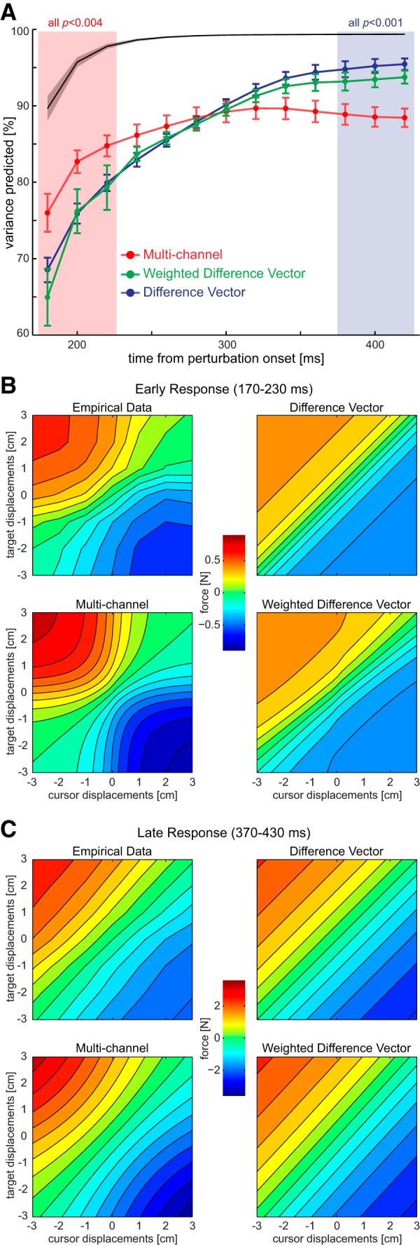
Time course of model fits. A, Predicted variance for the 36 combined conditions for each model as a function of the time from perturbation onset (±SEM). The black line indicates the noise ceiling, i.e., the maximal predictable variance given the intrasubject variance throughout the time. Shaded regions indicate the early and late time period from Figures 1 and 3. The p values above those quantify the comparison difference vector versus the multichannel model (two-sided t tests) B, Force responses during the early time window (170–230 ms after perturbation onset) plotted across all cursor and target displacements. Top left, Experimental data. Top right, Predicted responses of the difference vector model. Bottom left, Predicted responses from the multichannel model. Bottom right, Predicted responses from the weighted difference vector model. Note that each participant's equal-difference vector diagonals were monotonously increasing; only their average partially displays a nonmonotonous trend. Models are fitted to each subject's average data from isolated target and cursor perturbations, and the extrapolated predictions are shown for combined perturbations. C, Force responses during the late time window (370–430 ms after perturbation onset) and model predictions.