
Fig. 2. Bias correction.
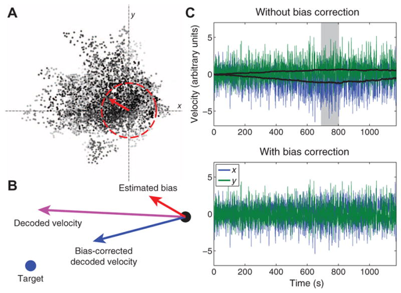
(A) Representative example of bias estimation, from 800 s into the first typing block of participant T7’s first self-paced typing session (trial day 293). At each moment in time, the direction and magnitude of the velocity bias (red arrow) were estimated by computing an exponentially weighted running mean of all decoded velocities (grayscale dots) whose speeds exceeded the 66th centile of the speed distribution (red dashed circle) computed from the previous filter build. This threshold was empirically found to be high enough to exclude low-velocity movements generated in an effort to counteract existing biases. The shading of each dot represents time, with darker dots occurring closer to the present moment [the end of the highlighted period in (C)]. (B) Effect of bias correction at the same moment displayed in (A). The location of the cursor is represented as a black dot. The location of the (retrospectively inferred) target is a blue dot. The red arrow represents the estimated bias at that moment in time [same as in (A)]. The purple arrow indicates the decoded cursor velocity at that moment before bias correction. The blue arrow indicates the bias-corrected velocity. (C) Effect of bias correction on this entire block of typing. (Top) Velocity traces with the estimated bias (black traces) added in. The gray box indicates the time interval when individual velocity samples are displayed in (A). (Bottom) Actual cursor velocities that occurred in session, bias correction having been continuously applied in real time.