Fig. 1.

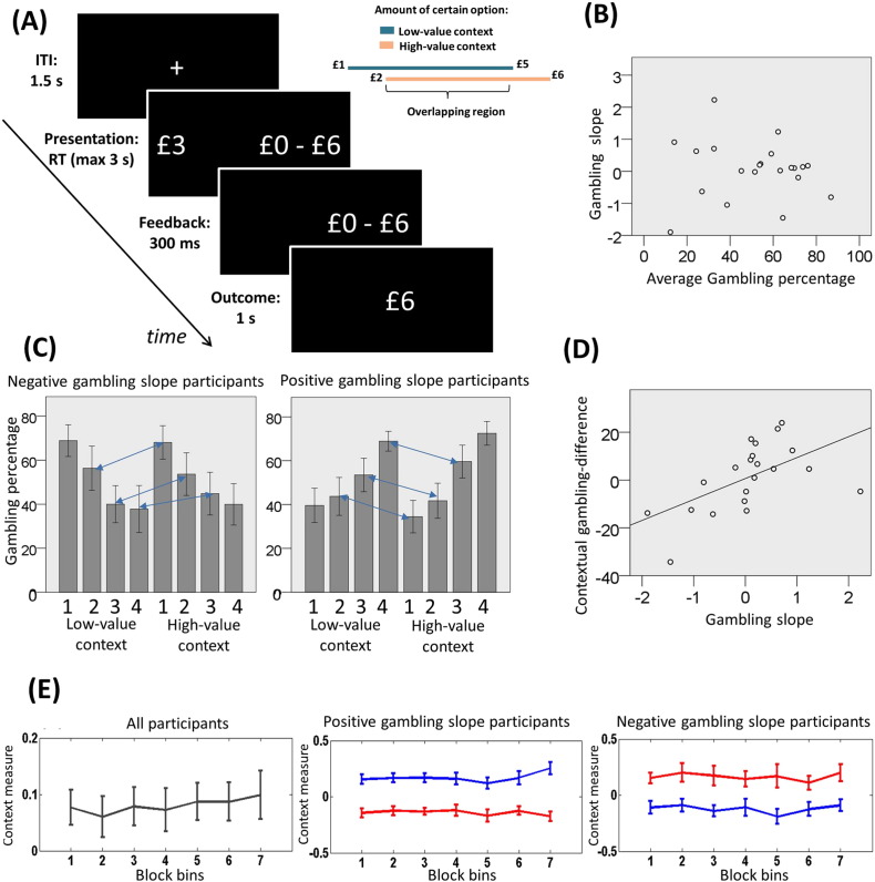
A: Experimental paradigm. Participants repeatedly made choices between certain gains (on the left in the example) and gambles (on the right in the example) associated with a 50% probability of either double the certain gain or zero. After a choice, the unchosen option disappeared and 300 ms later the trial outcome was shown for 1 s. The intertrial interval (ITI) was 1.5 s. At the end of the experiment, a single randomly chosen outcome was paid out to participants. B: Relationship between average gambling percentage (x-axis) and gambling slope (y-axis). This relationship was not significant (r(21) = − 0.06, p = 0.78, non-significant). Note that the gambling slope corresponds to the individual effect (i.e., the slope of a logistic regression parameter) of monetary amount on gambling, thus positive and negative gambling slopes correspond to increased gambling preference with increasing and decreasing amounts, respectively. A distribution of subjects (represented as dots) with positive and negative slopes is evident. C: Gambling percentage for different monetary amounts (grouped in 4 increasing magnitude bins: [1 2 3 4]) for each context (low and high). Participants are split in two groups based on their gambling slope (negative gambling slope: n = 9; positive gambling slope: n = 12). Blue arrows connect equivalent amounts presented in the two contexts. Consistent with a contextual normalization effect, subjects who gambled more with increasing amounts also gambled more when equivalent choices were relatively larger, that is in the low-value context. By contrast, subjects who gambled more with decreasing amounts also gambled more when equivalent choices were relatively smaller, that is in the high-value context. D: Relationship between gambling slope (x-axis) and contextual gambling difference for overlapping amounts (y-axis), corresponding to the gambling percentage in low-value minus high-value context for equal amounts (r(21) = 0.56, p = 0.008). E: Analysis of the evolution of the context effect over time. Blocks are separated into 7 bins. Values labelled as “context measure” represent an index of the context effect (see main text to see how this is obtained). Lines represent average across subjects and error bars represent standard error. The left panel combines all participants and shows that, after bins were aggregated in two sets (without considering the fourth bin), the values of the first three bins were overall not different from the values of the last three bins (t(20) = − 1.02; p = 0.319). Also, the value of the first bin was not significantly different from the value of the last bin (t(20) = − 0.758; p = 0.457) and was significantly larger than zero (t(20) = 2.46, p = 0.023). These data indicate that a context effect emerged from the very start of a new context presentation and remained stable across the duration of the block. On the middle and right panels, lines represent the risk preference for overlapping choices in the two contexts. Red and blue lines are for high- and low-value context, respectively. Participants are separated into two groups depending on whether they have a positive (middle panel) or negative (right panel) gambling slope.