Figure 1. Design and modeling of safeguard control in microbial swarmbots.

1. Design concept. Bacteria are engineered to exhibit collective survival. Bacteria confined in the microbial swarmbot can maintain a high local density and survive. Cells escaping the swarmbot will have a reduced density due to a larger extra‐capsule environment. If their density drops below their survival threshold, they will die, leading to safeguard control.
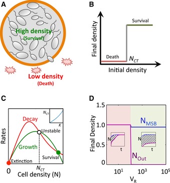
2. Collective survival. A population survives only when its initial density is > N_CT.
3. Simulation of collective survival. The collective survival can be described by a simplified model: $\frac{dN}{dt}=\mathit{\mu }N\left(1-\frac{N}{N_m}\right)-\left(\frac{d{K}^{\mathit{\alpha }}}{N^{\mathit{\alpha }}+K^{\mathit{\alpha }}}\right)N$, where μ is the maximum growth rate, N _m is the carrying capacity of the population, d is the maximum death rate of the cells, K is the critical threshold for survival, and α is the Hill coefficient. We assume that the growth rate of cells follows the logistic equation and that the death rate decreases with N. As the initial conditions, the parameters are set as N ₀ = variable from 0 to 1, μ = 1.75, N _m = 1, d = 2, K = 0.5, and α = 4. For the given parameter set, the system has three steady states. The trivial steady state (filled red circle) corresponds to extinction. The high state (filled green circle) corresponds to survival. Both are stable and are separated by an unstable steady state (N_CT, open circle). The population would reach the high steady state if and only if its density is greater than N_CT. The inset shows the correlation between N_CT and model parameter K.
4. Modulating safeguard with V_R. The effectiveness of safeguard can be quantified by the area under the curve (AUC) from density differences between the microbial swarmbot and the surrounding environment. The swarmbot dynamics can be described by a two‐compartment model: $\frac{d{N}_{\mathrm{MSB}}}{dt}=\mathit{\mu }{N}_{\mathrm{MSB}}\left(1-\frac{N_{\mathrm{MSB}}}{N_m}\right)-\left(\frac{d{K}^{\mathit{\alpha }}}{N_{\mathrm{MSB}}^{\mathit{\alpha }}+K^{\mathit{\alpha }}}\right)N_{\mathrm{MSB}}-f_N\left(N_{\mathrm{MSB}}-N_{\mathrm{Out}}\right),\text{and}\frac{d{N}_{\mathrm{Out}}}{dt}=\mathit{\mu }{N}_{\mathrm{Out}}\left(1-\frac{N_{\mathrm{Out}}}{N_m}\right)-\left(\frac{d{K}^{\mathit{\alpha }}}{N_{\mathrm{Out}}^{\mathit{\alpha }}+K^{\mathit{\alpha }}}\right)N_{\mathrm{Out}}+\frac{1}{V_R}{f}_N\left(N_{\mathrm{MSB}}-N_{\mathrm{Out}}\right)$, where the transport of cells between the two compartments is described by the final term in each equation. Modeling predicts that AUC increases with V_R, and once V_R becomes sufficiently large, AUC approaches infinity, indicating high level of safeguard. As the initial conditions, the parameters are set as follows: N_MSB  = 0.1 at t = 0, μ = 1.75, N _m = 1, d = 2, K = 0.01, α = 4, f_N = 0.1, V_R  = variable from 1 to 10⁵. Insets demonstrate the simulated growth dynamics for two representative V _R values.