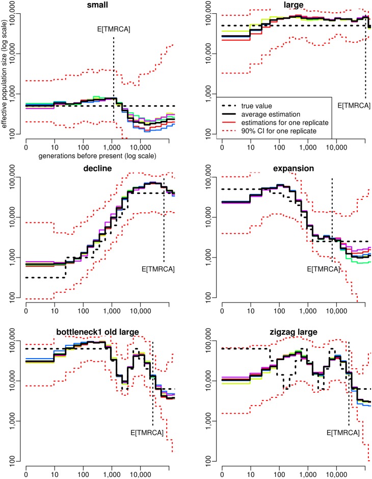
Fig 3. Estimation of population size history using ABC in six different simulated scenarios.

a small constant population size (N = 500, top left), a large constant population size (N = 50,000, top right), a decline scenario mimicking the population size history in Holstein cattle (middle left), an expansion scenario mimicking the population size history in CEU human (middle right), a scenario with one expansion followed by one bottleneck (bottom left) and a zigzag scenario similar to that used in [10] (bottom right), with one expansion followed by two bottlenecks. For each scenario, the true population size history is shown by the dotted black line, the average estimated history over 20 PODs is shown by the solid black line, the estimated histories for five random PODs are shown by solid colored lines, and the 90% credible interval for one of these PODs is shown by the dotted red lines. The expected time to the most recent common ancestor (TMRCA) of the sample, E[TMRCA], is indicated by the vertical dotted black line. Summary statistics considered in the ABC analysis were (i) the AFS and (ii) the average zygotic LD for several distance bins. These statistics were computed from n = 25 diploid individuals, using all SNPs for AFS statistics and SNPs with a MAF above 20% for LD statistics. The posterior distribution of each parameter was obtained by neural network regression [32], with a tolerance rate of 0.005. Population size point estimates were obtained from the median of the posterior distribution.