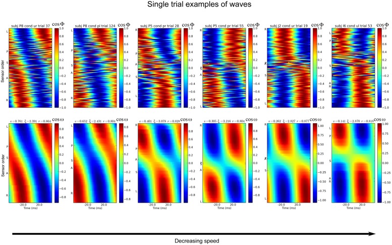
Fig 1. Examples of single trials with good fit to the wave model.

The top row shows the cosine of the phase, at 9.2 Hz, across all sensors. Examples are taken from a variety of subjects and experimental trials. The times shown on the x-axis are relative to the center time of one cycle of the wave. The bottom row shows the model wave that was fit to the data. v is the normalized velocity of the wave, ξ is the wavenumber (cycles/m) and r is the fit of the model wave to the data. On the y-axes, some sensors are labeled to indicate the approximate spatial ordering of the wave: ‘A’ is the most-anterior sensor, ‘P’ posterior, ‘I’ inferior, ‘S’ superior, ‘L’ left, and ‘R’ right. The sensors are ordered along the y-axis by values of the wave map calculated from the phases of the center time-sample.