Figure 4.

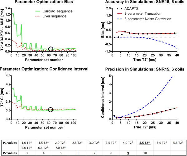
Parameter optimization from phantoms (left column and bottom table) and simulated optimal parameters of the ADAPTS method for the liver sequence TEs (right column). Parameter optimization: Top row shows how varying ADAPTS two parameters impacts bias, defined here as the mean difference between ADAPTS and the inline MLE method. Bottom row shows precision, measured as the CI size of 120 phantom measurements over different parameter values, together with the list of evaluated parameters. In both top and bottom rows, solid lines indicate measurements performed for the cardiac sequence and phantoms and the dashed lines indicate measurements from the liver sequence and phantoms. Circles show the selected parameter set used in the remaining parts of this study. The results indicate a robustness to variations in parameters above a threshold of approximately $P1$>3. Right column compares accuracy and precision of the optimized ADAPTS method with the two included signal models (truncation and noise‐correction) individually in simulations. The solid lines indicates the two‐parameter truncation method, the dashed line shows the three‐parameter noise correction method and the dotted line shows ADAPTS using the optimized parameter values. The optimized ADAPTS method balances low bias with maintained precision over the simulated T2* range. The shown simulations use TEs from the liver sequence, a SNR of 15, a ROI‐size of 40 and uses RSS reconstruction with six receive‐coils. The list of evaluated parameter values (bottom table) indicates the selected values of P1 and P2 with an underlined bold font.