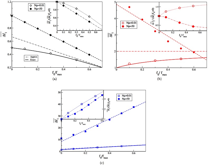
Fig 5. The main plot shows the fitness difference at the first step as a function of the initial fitness for various Nμ.

The fitnesses are chosen from Eq (1) with (a) κ = −1 (b) κ → 0 and (c) κ = 1/4. The solid lines in the main plot are obtained by numerically evaluating the integral given by Eq (9), while the dotted lines are the approximate results that can be obtained for the results when the initial fitness is high in the low mutation regime. The broken lines for κ ≠ 0 are lines of best fit as mentioned in the text. The broken line for κ → 0 is used for connecting the data points. The inset shows the fitness difference at the first step as a comparative measure of the fitness difference obtained at the first step when f₀ = 0. Here, the lines are used for connecting the data points.