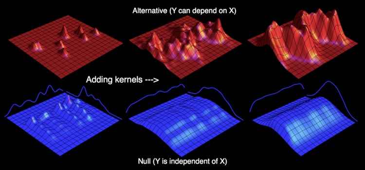
Fig 2. Estimating an unknown distribution.

The distribution for the alternative model (red—where X can depend on Y) is constructed by adding two dimensional Gaussian “kernel” distributions centered at each observation. As more of these kernels are added, the distribution comes to resemble the true distribution from which the observations are sampled. We can use a similar approach to estimating a null model that expressly disallows any dependence between X and Y (blue) by constructing one dimensional marginal distributions (the blue lines to either side) by summing one dimensional Gaussian kernels, and then creating the joint distribution as the product of these estimated marginals.