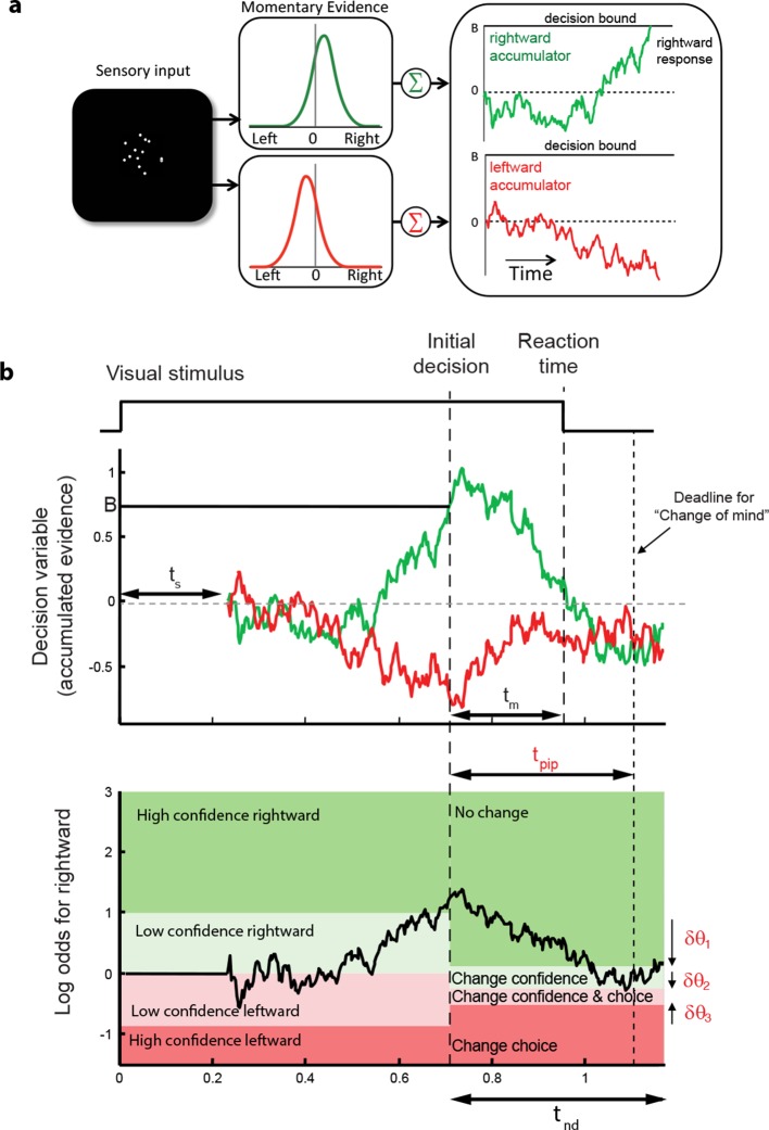
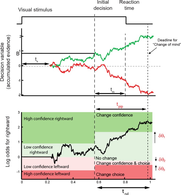
Figure 3. Information flow diagram showing visual stimulus and neural events leading to an initial decision, response time, and a possible change of mind.
(a) Competing accumulator model of the initial decision. Noisy sensory evidence from the random dot motion supports a race between a mechanism that accumulates evidence for right (and against left) and a mechanism that integrates evidence for left (and against right). Samples of momentary evidence are drawn from two (anti-correlated) Gaussian distributions with opposite means, which depend on the direction and motion strength of the stimulus. In this case the motion is rightward; therefore, the momentary evidence for right has a positive mean, and the rightward accumulator has positive drift. The first accumulation to reach an upper decision bound determines the choice and decision time. In this case the decision is for a rightward response. (b) Evolution of the decision variables (top) and log-odds (bottom) in the task. For simplicity we plot both accumulations on the same graph. At the initial decision time, the state of both the winning and losing processes as well as decision time confer the log-odds that a decision rendered on the evidence is likely to be correct, what we term confidence or belief. The bottom plot shows the log-odds of a rightward choice being correct, calculated from the decision variable and time. We assume that subjects adopt a consistent criterion θ on “degree of belief” to decide in favor of high or low confidence. Note that the decision is terminated by the decision variable (top), not the log-odds (bottom). Although the motion stimulus is displayed up to the reaction time, the decision does not benefit from all of the information, owing to sensory and motor delays (ts and tm, respectively). In the post-decision period, the accumulation therefore continues. Changes of confidence and/or decision are determined by which region the log-odds is in after processing for an additional time, tpip ≤ ts + tm. To incorporate energetics costs of changing a decision and having to reach mid-movement to a new target we allow the initial bounds to move from their initial levels (δθ1-δθ3). This example uses the parameter fits for Subject 1 and a 3.2% coherence with an initial high confidence correct rightward decision followed by a change of confidence to a rightward, low-confidence decision (for an initial low-confidence example see Figure 3-figure supplement 1).


