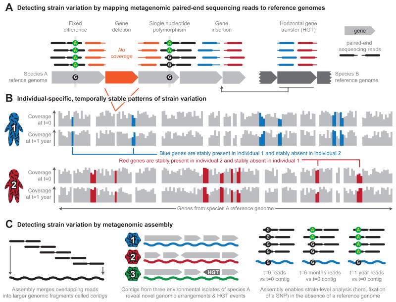
Figure 2. Profiling strain-level variation in microbial communities.

a. Mapping paired-end sequencing reads to microbial reference genomes reveals not only the genomes that are present in a community, but also differences between the isolates of particular species and the reference isolate. In this example, most positions have 4x coverage, represented by 4 paired-end sequencing reads stacked above (mapped to) each position in the reference genomes. Gene deletion events can be detected with relatively low coverage of the reference genome; deleted genes (in orange) recruit no reads from the sample and are flanked by paired reads (orange paired reads). Higher coverage facilitates differentiating between sequencing error and true nucleotide-level strain variation. Such variation includes fixed differences (in which the sample is consistently different from the reference at some site) and single nucleotide polymorphisms (SNPs; in which a site occurs in two or more states in the sample). Paired reads that do not map together (red and blue reads) indicate additional structural variation, including the insertion of genomic material not found in the reference by mechanisms such as horizontal gene transfer (HGT). b. Assembling paired-end reads into larger genomic fragments, called contigs, facilitates detection of strain variation in the absence of a reference genome. For example, analyzing contigs from three environmental isolates of a microbial species can reveal novel genomic arrangements and HGT events. Metagenomic assembly also allows the comparison of reference contigs (in this case, t = 0) to paired-end reads obtained at different time points during temporal analysis (such as t = 6 months or t = 1 year), which enables the identification of emerging SNPs. c. Mapping reads to reference genomes reveals patterns of gene presence and absence, which is a form of strain variation. Here, two individuals sampled at two time points (t = 0 and t =1 year) are distinguished by the presence and absence of genes in species A. The blue genes are stably present in individual 1 and stably absent in individual 2, whereas the red genes are stably present in individual 2 and stably absent in individual 1.