Figure 1.

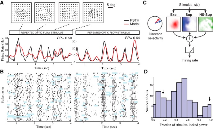
Response variability of MT neurons. A, The responses of two MT neurons to repeated presentations of a continuously varying optic flow stimulus, with four example frames from a section of the repeated stimulus segment (top). The peristimulus time histograms (PSTHs, bottom, black) are compared with the firing rate predictions of the stimulus-processing model (red), labeled with the fraction of stimulus-locked response explained by the model [predictive power (PP)]. B, Spike rasters of the same neurons as in A, from which the PSTHs are generated. The shaded areas mark epochs where data are excluded from analysis due to periods when eye position was outside the fixation window. C, Model schematic illustrating the main components of the stimulus-processing model: the stimulus composed is first processed locally by direction- and speed-selective local subunits, and then gets pooled across space separately by Exc (left), Sup (middle), and NS-Sup (right) components. Red and blue arrows (left) indicate direction selectivity for the Exc and Sup terms. Finally, a spiking nonlinearity is applied to this signal to transform it into a firing rate prediction (bottom). D, The distribution of the stimulus-locked rate variation across MT neurons (n = 108, mean = 45.9 ± 25.9%; see Materials and Methods). The black arrows indicate the location of the two example neurons in A (stimulus-locked variance = 16.5% and 96.4%).