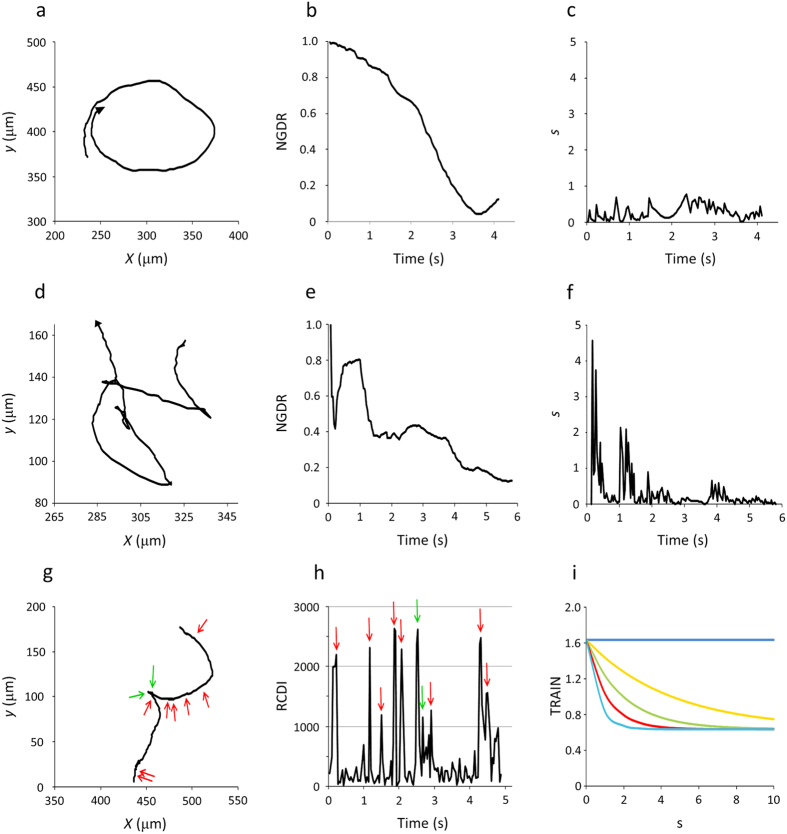
Figure 4. Illustration of different components of the trajectory index (TRAIN).

In (a,d), two trajectories with low NGDR are compared. (a) Smooth circular trajectory (wild-type, NGDR = 0.12). (d) Irregular trajectory (ΔlafA, NGDR = 0.13). In each one, the rate of change of NGDR over time is different, being mild in the smooth trajectory (b) or steep in the irregular trajectory (e), giving rise to low (c) or high (f) absolute values of the maximal slope (s). (g) A trajectory of ΔlafA with an RRF showing the two changes in direction (green arrows) that were correctly predicted as RCDI > 1,000 (h), although there were 8 false positives in positions with RCDI > 1,000 but no apparent change in direction (red arrows). (i) Generic variation of TRAIN. In the graph, the values of <cos α> and c were fixed at 0.8 and 2, respectively, and NGDR was considered as 1.0 (blue), 0.8 (orange), 0.6 (green), 0.4 (red) or 0.2 (light blue). Hence, these curves depict the variation of TRAIN with NGDR and s when <cos α> and c are fixed, but because the curves were obtained from y = a + b^x, they can also illustrate how TRAIN varies with <cos α> and c when NGDR and s are fixed. The coordinate values in (a,d,g) correspond to those of Fig. 2a–d.