Extended Data Figure 8. The potential effects of heterogeneity at 33 °C.

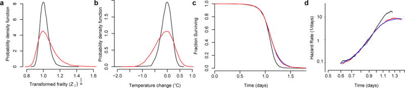
a, Fifty-six thousand samples were drawn from the distribution of frailty effects Z^−1/α as described in Supplementary Note 3.1, where Z is a random variable, sampled from an inverse-gamma distribution with mean 1 and a standard deviation corresponding to the value estimated from experimental data. Samples were drawn using the σ² estimated for populations at 25 °C (black) and at 33 °C (red), corresponding to the data presented in Fig. 1d. The probability density function of each population is shown, which can be interpreted as the variable effect of unknown factors on lifespan across individuals at each temperature. b, At each temperature, 25 °C (black) and at 33 °C (red), we estimated the distribution of temperature changes required to produce the distribution of frailties shown in a. This was accomplished using temperature scaling function shown in Fig. 4b. c, Fifty-six thousand random samples were drawn from the transformed inverse gamma distribution of Z^−1/α with σ² set to the estimate of Δσ² in equation (15) of Supplementary Note 3.2. Each sample was multiplied by a death time drawn (with replacement) from the set of 25 °C residual times of Fig. 1d, shown here in black. These products constitute a ‘transformed’ set of death times, corresponding to the 25 °C residuals with additional frailty synthetically introduced. The residual death times of animals placed at 33 °C are shown for comparison (red).