Figure 4.

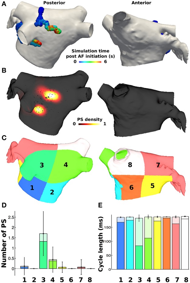
PS locations during pAF from LSPV pacing. (A) PS trajectories on the posterior (shown on the left) and anterior (shown on the right) walls, colored by time (ms) during the simulation post LSPV pacing. (B) Spatially smoothed PS density map, indicating rotors localized only in the area of high fibrosis density on the posterior wall. (C) Eight LA subdivisions were used for analysis and correspond to the LA location numbers in Figure 6. (D) Regional assessment of the mean and standard deviation of PSs and the mean number of rotors (shown in a darker shade) over the duration of the simulation show that subdivision 3 has the highest PS density. (E) Regional assessment of average CL for each vertex in the pAF bilayer model indicates that mean average CL is constant across subdivisions, while the minimum average CL varies (shown in a darker shade).