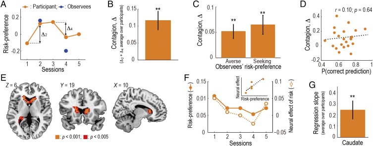
Fig. 2.

Contagion of risk-preference. (A) Change of an example participant’s risk-preference toward the observees’. Orange indicates the participant’s risk-preference in each session, and blue indicates the observees’ preference. The degree of contagion is defined as Δ: the change of the risk-preference (i.e., proportion of gambles accepted) from the last session. Δ is positive when the participant conformed to the observee; negative when she/he anticonformed. (B) Degree of contagion (mean $\pm$ SEM across participants, n = 24). The degree, Δ, is defined as the sum of Δ₂ and Δ₄. **P < 0.01. (C) Degree of contagion plotted separately for the risk-averse and -seeking observees (mean $\pm$ SEM across participants). (D) Degree of contagion in each participant plotted as a function of the proportion of the correct predictions made on Predict trials. (E) Neural representation of risk. Activity in the caudate significantly correlated with risk of the gamble at the time of decision in Self trials [P < 0.05 FWE corrected at cluster-level; GLM I (SI Methods)]. (F) Relation between the behavioral risk-preference and the neural effect of risk in the caudate in an example participant. Filled points indicate the participant’s behavioral risk-preference in each session; open points indicate the neural effect of risk (i.e., β value for the risk regressor in GLM I) in each session. (Inset) Scatter plot of the same data. (G) Relation between the behavioral risk-preference and the neural effect of risk (mean $\pm$ SEM across participants). We regressed the neural effect in the caudate against the behavioral risk-preference across sessions and plot the average regression coefficient over the participants.