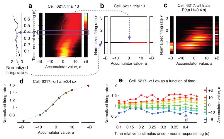
Figure 2. Computing tuning curves that describe the relationship between neural activity and accumulated evidence.

a, One trial for an example neuron from PPC. The left side shows the neuron’s firing rate, and the right side shows the behavioral model’s estimate of the evolution of the distribution of a (color represents probability density). Time runs vertically and is aligned to stimulus onset minus neural response lag. ±B correspond to the “sticky” decision-commitment bounds on evidence accumulation. b, Building a map of firing rate versus accumulator value. At a given timepoint (here, t=0.4), we copy the distribution of a (purple box) to a vertical position given by the neuron’s firing rate. c, Continuing with the same timepoint, we add a slice from very recorded trial. This produces the full joint distribution P(r,a | t=0.4), the probability of seeing firing rate r and accumulator value a at time t=0.4. d, The accumulator values are binned, and mean firing rate is computed for each bin to generate a neural tuning curve as a function of a. e, The process is repeated for each timepoint. Each vertical slice corresponds to a tuning curve, with the one from panel (d) shown above the purple arrowhead.