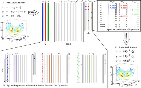
Fig. 1.

Schematic of the SINDy algorithm, demonstrated on the Lorenz equations. Data are collected from the system, including a time history of the states $\mathbf{X}$ and derivatives $\dot{\mathbf{X}}$; the assumption of having $\dot{\mathbf{X}}$ is relaxed later. Next, a library of nonlinear functions of the states, $\mathrm{\Theta }\left(\mathbf{X}\right)$, is constructed. This nonlinear feature library is used to find the fewest terms needed to satisfy $\dot{\mathbf{X}}=\mathbf{\Theta }\left(\mathbf{X}\right)$Ξ. The few entries in the vectors of Ξ, solved for by sparse regression, denote the relevant terms in the right-hand side of the dynamics. Parameter values are $\sigma =10,\beta =8/3,\rho =28$, ${\left(x_0,y_0,z_0\right)}^T={\left(-\mathrm{8,7,27}\right)}^T$. The trajectory on the Lorenz attractor is colored by the adaptive time step required, with red indicating a smaller time step.