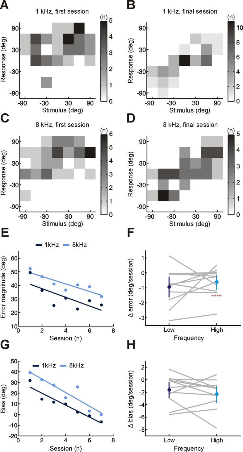
Figure 2. Effect of training on localization of pure tone stimuli in the horizontal plane by monaurally deprived human listeners.

(A–D) Joint distributions of stimulus and response obtained from the first (A,C) and last (B,D) training sessions for low- (A,B) and high-frequency (C,D) tones. Data are shown for an individual subject wearing an earplug in the left ear, with grayscale indicating the number of trials corresponding to each stimulus-response combination. Because pure tones can be accurately localized only by using binaural spatial cues, which are susceptible to front-back errors, data from the front and rear hemifields have been collapsed. (E) Mean error magnitude plotted as a function of training session for the same subject shown in A–D. Data are plotted separately for low- (1 kHz, dark blue) and high-frequency (8 kHz, light blue) tones. Scores for each session (dots) were fitted using linear regression (lines) to calculate slope values, which quantified the change in error magnitude (Δ error) with training. Improved performance was associated with a reduction in error magnitude, producing negative values for Δ error. (F) Δ error for low- and high-frequency tones plotted for each subject (gray lines; n = 11). Mean values for Δ error across subjects (± bootstrapped 95% confidence intervals) are shown in blue. Although there are pronounced individual differences for the adaptation observed at the two tone frequencies, almost all values are <0, indicating that error magnitude declined over the training sessions. Dotted red line shows Δ error values that would have been observed if subjects had adapted as well as ferrets reared with a unilateral earplug (Keating et al. 2015; total Δ error reported for ferrets was divided by the number of training sessions used in the present study, n = 7; normalization used in previous work has been removed to facilitate comparison). (G) Bias in sound localization responses plotted as a function of training session for the subject in E. Positive values indicate that responses were biased toward the side of the open ear. Data are plotted separately for low- (1 kHz, dark blue) and high-frequency (8 kHz, light blue) tones. Scores for each session (dots) were fitted using linear regression (lines) to calculate slope values, which quantified the change in response bias (Δ bias) with training. Negative values of Δ bias indicate a shift in response bias toward the side of the plugged ear. (H) Δ bias for low- and high-frequency tones plotted for each subject (gray lines; n = 11). Mean values for Δ bias across subjects (± bootstrapped 95% confidence intervals) are shown in blue.
