Figure 2.

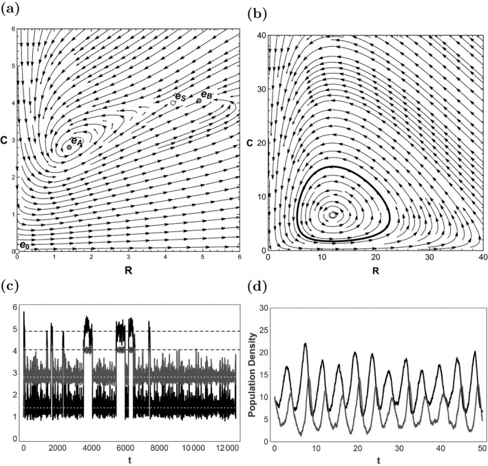
(a) Stream plot for the deterministic skeleton of the consumer‐resource model in example 2. Unstable equilibria are white disks and stable equilibria are gray disks. The unstable equilibrium ${\mathbf{e}}_P$ is not shown, but would appear on the x‐axis to the right of where the graph is truncated. Variables are scaled, so the units are dimensionless. Lines and arrows show the direction of trajectories for Eq. (8) in the absence of noise. (b) Similar stream plot for the deterministic skeleton of the consumer‐resource model in example 3. The white disk is an unstable equilibrium and the gray line is a stable limit cycle. (c) A realization of Eq. (8) for example 2. Integration was performed with the Euler‐Maruyama method and Δt = 0.025. Resource population density is black and consumer population density is gray. The dotted white lines correspond to the equilibrium ${\mathbf{e}}_A$, and the dashed black lines to the equilibrium ${\mathbf{e}}_B$. (d) A realization of Eq. (15) for example 3, with σ = 0.8. Integration was performed with the Euler‐Maruyama method and $\mathrm{\Delta }t=5\times {10}^{-4}$. Resource population density is black and consumer population density is gray.