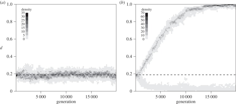
Figure 1.

Examples of dispersal distributions through time in model M₁ for symmetric (a) and asymmetric metacommunity (b) respectively (see table 1 for metacommunity features). One simulation run is represented in each panel. The grey shades refer to individuals' density when all species are pooled together (null in the white areas). Time is given in generation numbers. Parameters describing dispersal evolution are μ = 0.01 and σ = 0.01, and the cost of dispersal is c = 0.1.