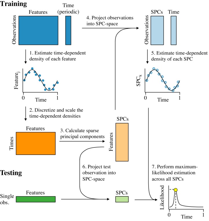
Figure 1.

Schematic of the ZeitZeiger algorithm. The periodic variable is denoted as ‘time,’ with values between 0 and 1 and time = 0 equivalent to time = 1. Training data consist of a matrix of measurements for observations by features and a corresponding time for each observation. (1) The time-dependent mean of each feature is estimated as a smooth periodic spline and the variance about the mean is estimated based on the residuals. (2) A new matrix is constructed, in which the time-dependent mean of each feature is discretized into a number of time-points and scaled by that feature's standard deviation about the mean curve. (3) Sparse principal components (SPCs) of the new matrix are calculated. (4) The loadings of the features for each SPC are used to project the training data from feature-space into SPC-space. (5) The time-dependent mean and the variance of each SPC are estimated using the same procedure that was used for the features. (6) Each test observation is projected from feature-space into SPC-space. (7) Given the SPC values of the test observation and the time-dependent densities of the SPCs from the training data, the time of the test observation is predicted using maximum-likelihood.