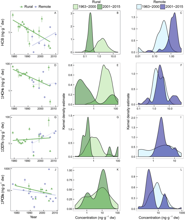
Figure 4. Individual relationships among HCB, ΣHCHs, and ΣDDTs (ng·g−1 dry weight) and year.
The equations for rural and remote areas are: (A) HCB rural: y = −0.04× + 91, r2 = 0.19, df = 1354, P < 0.0001, and HCB remote: y = 0.07× − 140, r2 = 0.43, df = 1,95, P < 0.0001; (D) ΣHCHs rural: y = −0.07× + 148, r2 = 0.31, df = 1,356, P < 0.0001, and ΣHCHs remote: y = 0.08× − 16, r2 = 0.01, df = 1,143, P = 0.2; (G) ΣDDTs rural: y = −0.01× + 23, r2 = 0.01, df = 1,356, P = 0.09, and ΣDDTs remote: y = 0.01× − 13, r2 = 0.00, df = 1,155, P = 0.4; and (J) ΣPCBs rural: y = −0.02× + 50, r2 = 0.11, df = 1,102, P < 0.001, and ΣPCBs remote: y = −0.03× + 71, r2 = 0.24, df = 1,124, P < 0.0001. Panels (B), (E), (H) and (K) and (C), (F), (I) and (L) show the estimated curve for kernel density for both rural and remote regions, respectively, before and after 2000.

