Figure - PMC

Skip to main content

An official website of the United States government

Here's how you know

Here's how you know

Official websites use .gov
A .gov website belongs to an official government organization in the United States.

Secure .gov websites use HTTPS
A lock ( ) or https:// means you've safely connected to the .gov website. Share sensitive information only on official, secure websites.

View full-text article in PMC

. 2015 Oct 9;124(5):619–626. doi: 10.1289/ehp.1509761

Search in PMC
Search in PubMed
View in NLM Catalog
Add to search

Publication of EHP lies in the public domain and is therefore without copyright. All text from EHP may be reprinted freely. Use of materials published in EHP should be acknowledged (for example, “Reproduced with permission from Environmental Health Perspectives”); pertinent reference information should be provided for the article from which the material was reproduced. Articles from EHP, especially the News section, may contain photographs or illustrations copyrighted by other commercial organizations or individuals that may not be used without obtaining prior approval from the holder of the copyright.

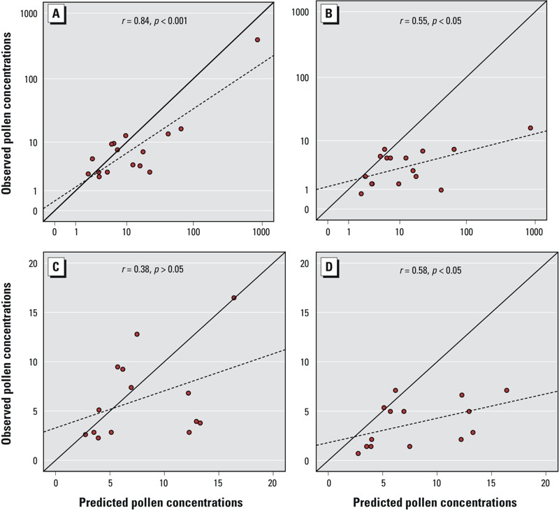
PMC Copyright notice

Scatter plots of the observed (i.e., measured) and predicted grass pollen concentrations (grains/m³) for the larger (n = 16) (A,B) and smaller (n = 14) (C,D) data sets. In the evaluation setting, the observed concentrations were measured during morning (0800–1130 hours, 27 June–9 July 2013) (A,C) and another period (0800–1130 and 1300–1630 hours, 10–21 July 2013) (B,D). The solid line shows the optimum fit (intercept = 0, slope = 1) and the dashed line the fit to the data. Pearson’s correlation coefficients (r) are also shown.