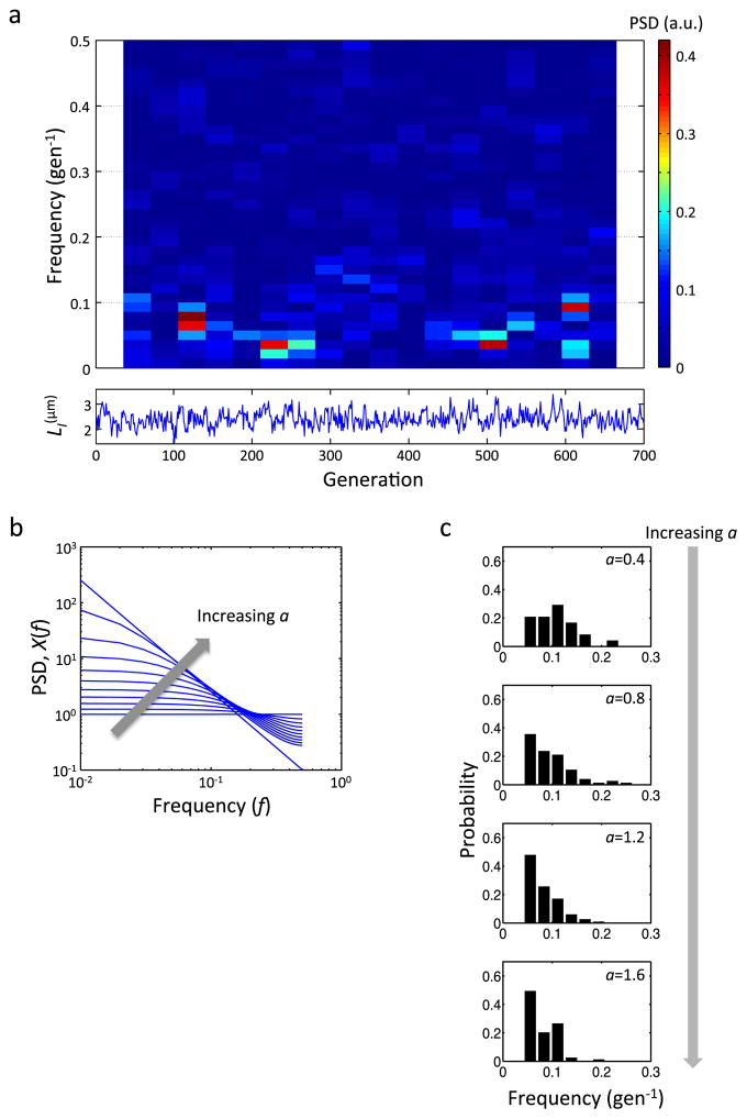
Extended Data Figure 3. Frequency analysis of noisy linear map.

a, Time-frequency analysis of the noisy linear map model for L_I. The upper panel shows a spectrogram of 700-generation simulation constructed using 70-generation segments with 50% overlap. The lower panel shows the temporal dynamics of L_I. The same parameters as in Fig. 2a were used. b, The power spectrum of noisy linear map (X(f)). Eq. 3 is plotted for different a (0 ≤ a ≤ 1.8 with 0.2 interval). X(f) = 1 / (2πf)² for a = 2 is the straight line in this log-log plot. Note that the maximum value of f is 0.5 as the time resolution is 1 generation. c, Dependence of oscillation frequencies on a simulated using the rescaled linear map (Eq. 2). The noisy linear map model was simulated (Fig. 3a–c) and the distributions of oscillation frequencies are shown for four different values of a (from top to bottom, n = 24, 76, 117, and 79, respectively).