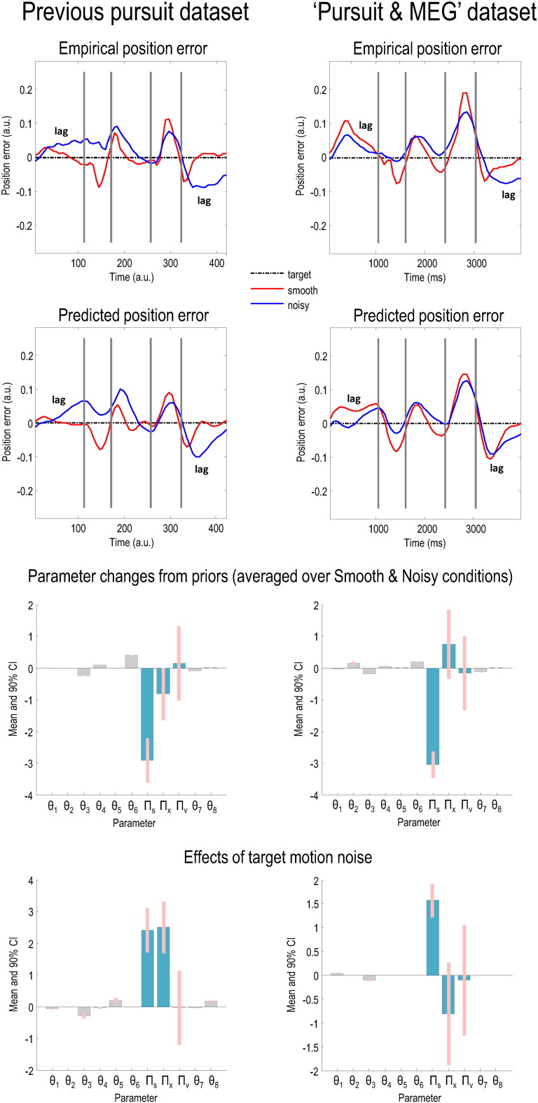
Fig. 6.

Comparison of empirical and predicted position errors and parameter estimates in this and a previous dataset.

The graphs on the first row show empirically observed position error (target position — eye position) in arbitrary units (the traces have been normalised with respect to displacement) for both Smooth (red line) and Noisy (blue line) conditions. Note that being behind the target entails being above the black line in the first half of the cycle and below it in the second. It is clear that the pattern of eye movements in each condition is very similar in both experiments; the major difference is an increase in lag in the Smooth condition in the second experiment, especially in the first quarter cycle (please see the main text for discussion of this phenomenon). The graphs on the second row show the position errors predicted by the generative model in Fig. 1, using the posterior expectations of the parameters in the lower two rows: in both experiments, the models fit the data well. The previous experiment (left panels) used two different speeds and hence the plots on the left have been normalised with respect to time, but those on the right – using only one speed – have not.

The graphs on the third and fourth rows depict the parameters used to generate the predicted position errors on the second row. The graphs on the third row display the posterior expectations of the model parameters (averaged over conditions), plotted as the changes from prior expectations listed in Table 1. The graphs on the fourth row display the changes in parameters due to the noise of target motion. The changes in kinetic parameters (θ₁, …, θ₆) are absolute, but the changes in precision parameters (teal) and prior parameters are log scaled. The pink bars correspond to 90% Bayesian confidence intervals. The posterior expectations in each dataset are remarkably similar: please see the text for a discussion of their minor differences.