
Figure 3. Computational model.
(A) Schematic illustration of the computational model. FG domains are represented as end-grafted polymers anchored at 5.5 pmol/cm2 (i.e., 3.3 molecules per 100 nm2) to the bottom of a 100 nm diameter cylinder, and modeled as strings of beads, where each bead has equal bond length and diameter (two amino acids, 0.76 nm). The number of polymer beads was set to match the length of experimentally used FG domains. NTF2 dimers and Impβ are represented as spherical colloids of 4.0 and 6.0 nm diameter, respectively. (B) Matching of the computational model with experimental data for FG domain films in the absence of NTRs. Horizontal lines represent the experimentally determined film thickness per amino acid for different FG domains (black line - Nsp1 at 4.9 pmol/cm2; blue line - Nup98-glyco at 5.4 pmol/cm2; orange line - reg-FSFG at 6.1 pmol/cm2), with shaded areas in matching colors indicating confidence intervals. Symbols represent the thickness as predicted by the computational model as a function of εpp for the different FG domains (at 5.5 pmol/cm2; colors match experimental data). The data points and the upper and lower ends of the vertical lines refer to the effective thicknesses where the densities have dropped to 5%, 1% and 10% of the maximal densities in the film, respectively. Symbols for Nsp1 and Nup98-glyco are translated along the x axis by +0.1 kBT and -0.1 kBT, respectively, to improve their visibility. Dashed lines through the symbols are cubic interpolations (the black dashed line is for Nsp1 and Nup98-glyco). Full computational details are available in ‘Materials and methods’ and Figure 3—figure supplements 1–5.
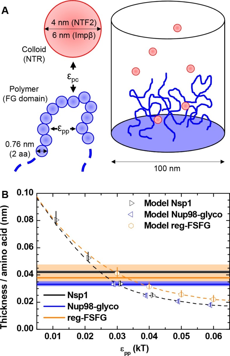
Figure 3—figure supplement 1. Scheme illustrating how computational modeling data is presented in the form of maps of the polymer and colloid packing fractions.
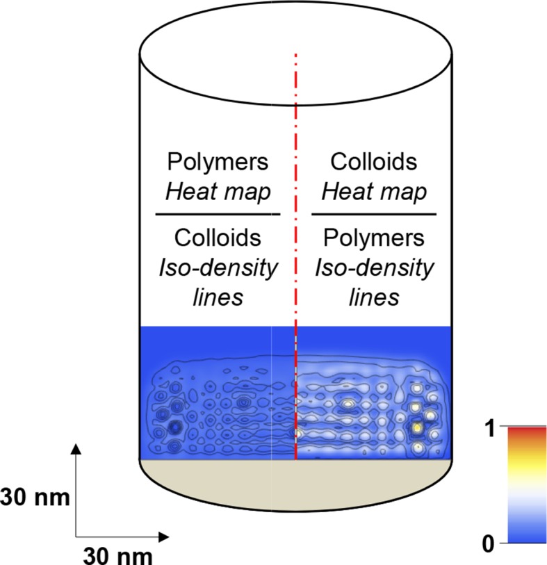
Figure 3—figure supplement 2. Computational modeling data for a polymer length equivalent to Nsp1 and colloids of 4.0 nm diameter (equivalent to NTF2 homodimers).

Figure 3—figure supplement 3. Computational modeling data for a polymer length equivalent to Nup98-glyco and colloids of 4.0 nm diameter (equivalent to NTF2 homodimers).

Figure 3—figure supplement 4. Computational modeling data for a polymer length equivalent to reg-FSFG and colloids of 4.0 nm diameter (equivalent to NTF2 homodimers).

Figure 3—figure supplement 5. Computational modeling data for a polymer length equivalent to Nsp1 and colloids of 6.0 nm diameter (equivalent to Impβ).
