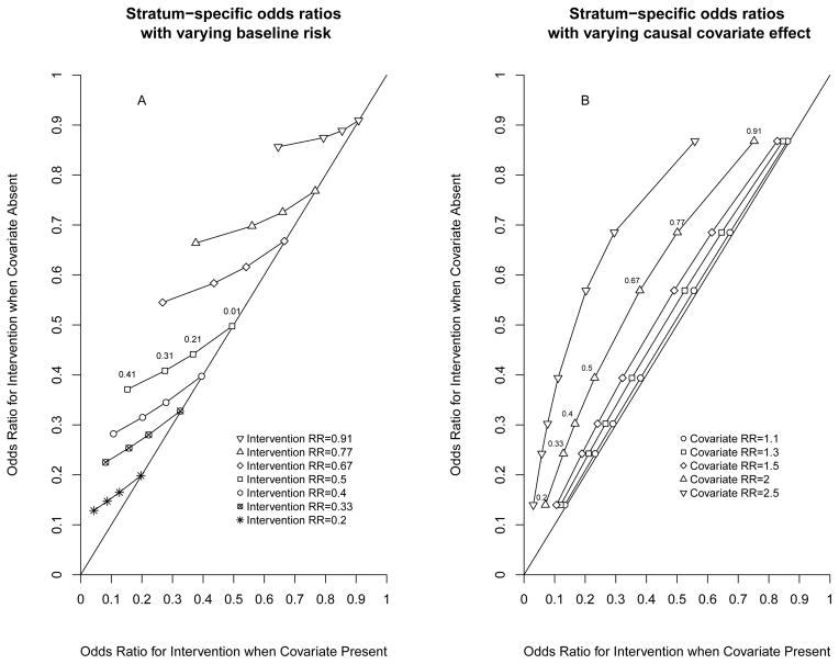
Figure 2.

Graphs illustrating how stratum specific odds ratios (OR) will differ even when there is no bias or causal effect modification. In both panels, the OR for the intervention when the covariate is absent (y-axis) is plotted against the OR for the intervention when the covariate is present (x-axis). Any deviation from the line of identity on the graph means that the OR in the two different strata are different. In A, the effect of the covariate is held constant and doubles the risk of the outcome. Each set of symbols represent a particular relative risk (RR) for the intervention, but at increasing baseline risks from 0.01 (rightmost point) to 0.41 (leftmost point). The difference between the stratum-specific OR increases as the baseline risk increases, and as the RR increases, but is negligible at very low baseline risks. In B, the baseline risk under control conditions in the absence of the covariate is held constant at 35%. Each set of symbols represents a particular strength for the covariate effect (e.g. upright triangles Covariate RR=2 mean the covariate doubles the risk of the outcome), with each symbol representing the OR at intervention RR ranging from 0.2 (lowest point) to 0.91 (highest point). The difference between stratum-specific OR increases as the strength of the covariate increases (from left to right). Because the baseline probability is held constant at 35%, the maximum covariate RR shown is 2.5 (e.g. covariate RR=3 would give an impossible probability of 1.05).