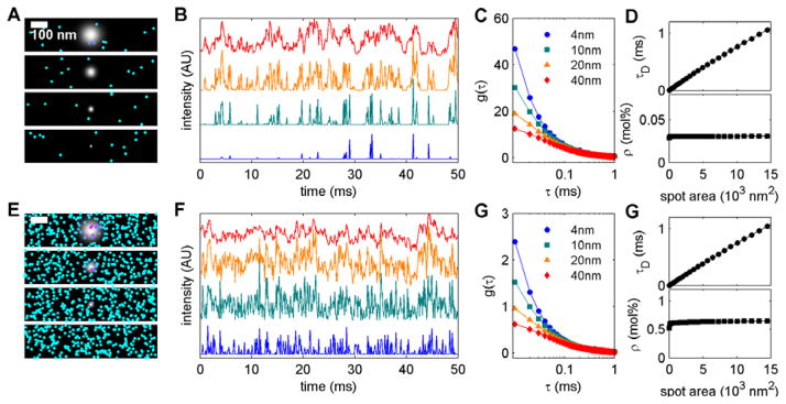
Figure 1. Simulating spot size dependent correlation functions for Brownian motion.
(A,E) Representative snap-shots of simulations conducted at low (A; 0.03%) and high (E; 0.6%) tracer densities. Tracers are drawn larger than their actual size for demonstration purposes. Images also depict the size and shape of several Gaussian illumination spots (40, 20, 10, and 4nm) standard deviations going from top to bottom. (B, F) Representative time-traces calculated by superimposing the illumination spot on the tracer distribution as described in Methods. Traces correspond to the same illumination areas and order shown in A, E. (C,G) Time-time autocorrelation functions, g(τ), tabulated from time-traces like those shown in B,F. The points shown are an average over multiple spot locations and simulations, and error bounds are smaller than the point dimensions. Lines are fits to Eqn 3 which describes Brownian motion in two dimensions. Fits report the mean transit time, τD, and the number of tracers per spot, N. (D,G) Plots of fit parameters vs. illumination area. τD varies linearly with area and intersects the origin, as expected for Brownian motion. The slope of this line is related to the diffusion coefficient as D = 1/(4 × slope) = 3.4μm2/s. N is converted into a % of tracers, ρ, which is independent of spot area, where ρ=N/(spot area) ×(box area)/(total number of components) ×100%. Simulations were conducted in the Ising model with T = 5×TC

