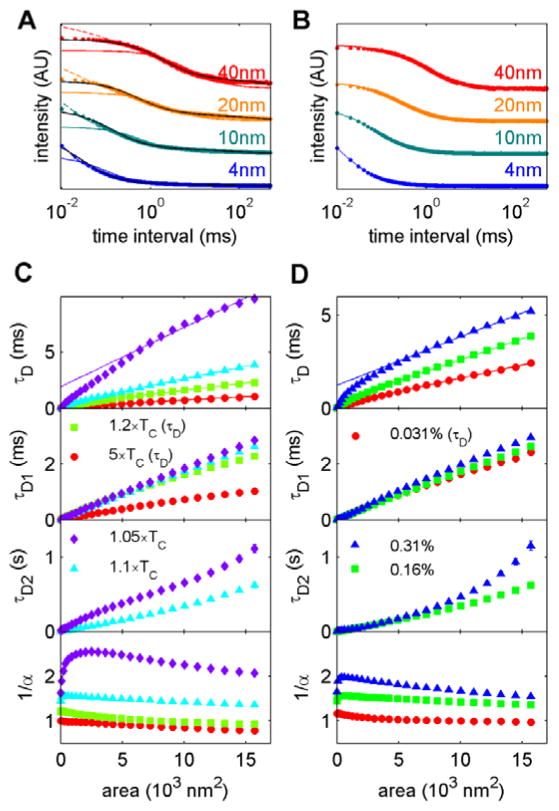
Figure 3. Fit parameters from simulated g(τ).
(A) Aggregate g(τ) curves from simulations conducted with T = 1.1×TC and ρ=0.16% and the indicated illumination half-widths (σ). Lines are fits to a single Brownian population (Eqn 3; solid color), two Brownian populations (Eqn 4; solid black) and a single anomalous population (Eqn 5; dash color). (B) g(τ) curves for T = 5×TC and ρ=0.16% at the same illumination half-widths. Solid line is a fit to a single Brownian population (Eqn 3). (C) Summary of fit parameters obtained for ρ=0.16% over the range of temperatures indicated. Fit parameters are described in Eqns 3–5 in Methods. At high temperatures, the four parameter fit of Eqn 4 is not well specified, therefore τD is replotted for τD1 and τD2 is not plotted for these conditions (T = 1.5×TC, 5×TC). (D) Summary of fit parameters obtained for T = 1.1×TC over the range of tracer densities indicated. At the lowest tracer density shown τD is replotted for τD1 and τD2 is not plotted for (ρ=0.03%) because the fit to Eqn 4 was not well specified. The solid line in plots of τD vs area in C,D is a linear fit to τD points corresponding to areas between 5.6×10³ and 1.6 ×10⁴ nm2. This line is extrapolated to area=0 to illustrate the positive y intercept.

