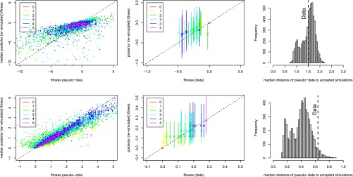
Figure 4.

Posterior predictive checks on two example data sets. One data set is compatible with Fisher’s model (top row; Aspergillus data set A1), and one rejects Fisher’s model (bottom row, data set F). (Left) The median posterior fitness against the “true” fitness of pseudodata generated under Fisher’s model for the cross-validation showing that when the pseudodata have been generated using Fisher as the true model, the posterior fitnesses are close to the true fitness values. (Center) Posterior predicted log-fitness as a function of the true experimental log-fitness. The points are the median posterior, and the lines show the 2.5–97.5% interval. The color code indicates the number of mutations of each genotype, the ancestor in red being set to log-fitness = 0. The median posterior fitnesses are very well correlated with the true fitnesses when the landscape is compatible with Fisher’s model but less so when Fisher’s model is rejected. (Right) The median distance of pseudodata to the accepted simulations when the pseudodata are simulated under Fisher’s model and the posterior parameters. This distribution together with the observed median distance for the experimental data (dashed line) is used to calculate the P-value corresponding to the null hypothesis: “the underlying fitness landscape is Fisher’s model.”