Figure 2.

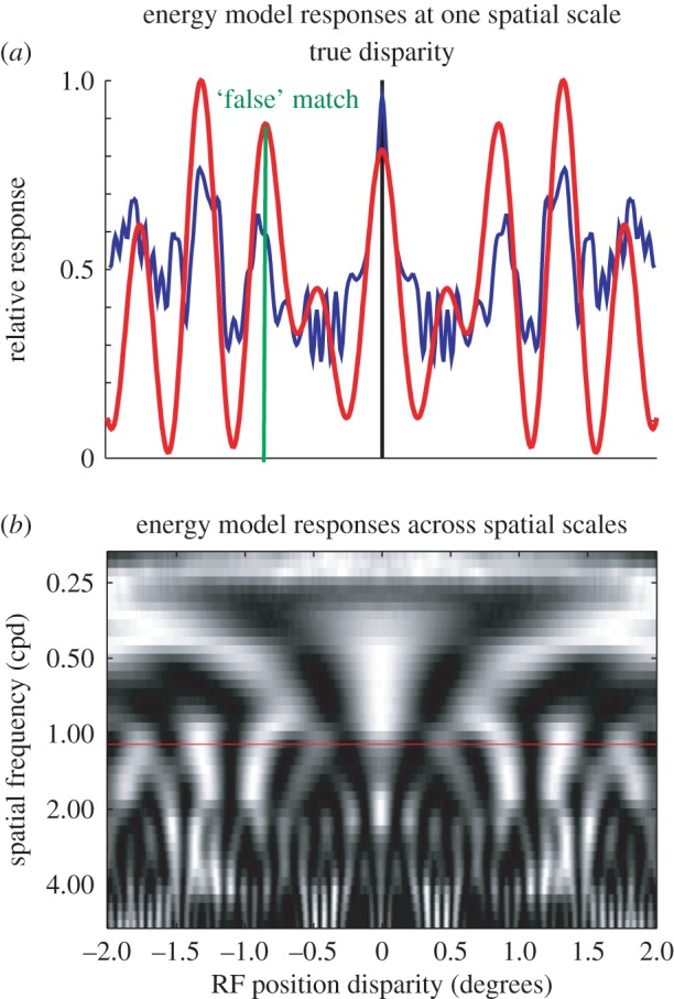
The correspondence problem after filtering with the binocular BEM, represented by considering the response of a population of model complex cells to a single binary noise pattern. This pattern has zero disparity—the image is identical in both eyes. This simulation was run using the one-dimensional RFs shown in figure 1, with one-dimensional images. The image pixel size was 0.005° (100 pixels per cycle of the carrier). (a) The response profile across a population of neurons that differ only in their position disparity (smooth red curve; equivalent to the responses of the complex cell shown in figure 1 to different disparities). The position disparities were introduced by displacing the RFs in each eye symmetrically, so the mean (cyclopean) RF position is constant. There is a local maximum at the true disparity, but several other local maxima—‘false’ matches. The false matches can have a greater magnitude than the response to the true disparity. (b) A population differing in both position disparity and spatial scale (quantified by the preferred spatial frequency). The colour scale shows relative response (like the ordinate in (a)), in which each horizontal row has been normalized to a maximum of unity. The red horizontal line marks the set of model cells used in (a). Note that while every row in this image has a local maximum at the true disparity, the locations of the false matches depend on the spatial scale of the filters. Consequently, a simple summation across spatial scales can extract the correct disparity in most cases. The blue (less smooth) line in (a) shows this sum normalized (like the smoother red curve) to a maximum of unity. Note that here the global maximum is at the true disparity.