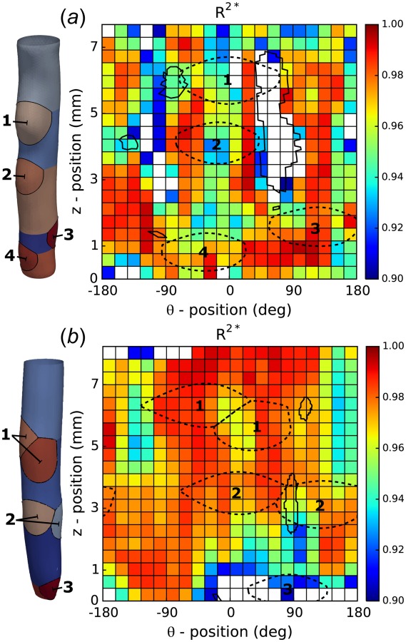
Fig. 2.

Spatial distribution of the coefficients of determination. Goodness-of-fit for (a) specimen A and (b) specimen B. Both panels show outputs from a modified branch splitting algorithm to highlight regions of influence due to specimen branches (1–4). The results are shown in both a 3D (left) and 2D (right) representation over the entire surface of each sample. Boundaries of both low mean curvature (solid enclosed regions) and regions of branch influence (dashed ellipses) are overlaid in the 2D representation to show localization with regions of low .
