Fig. 5.

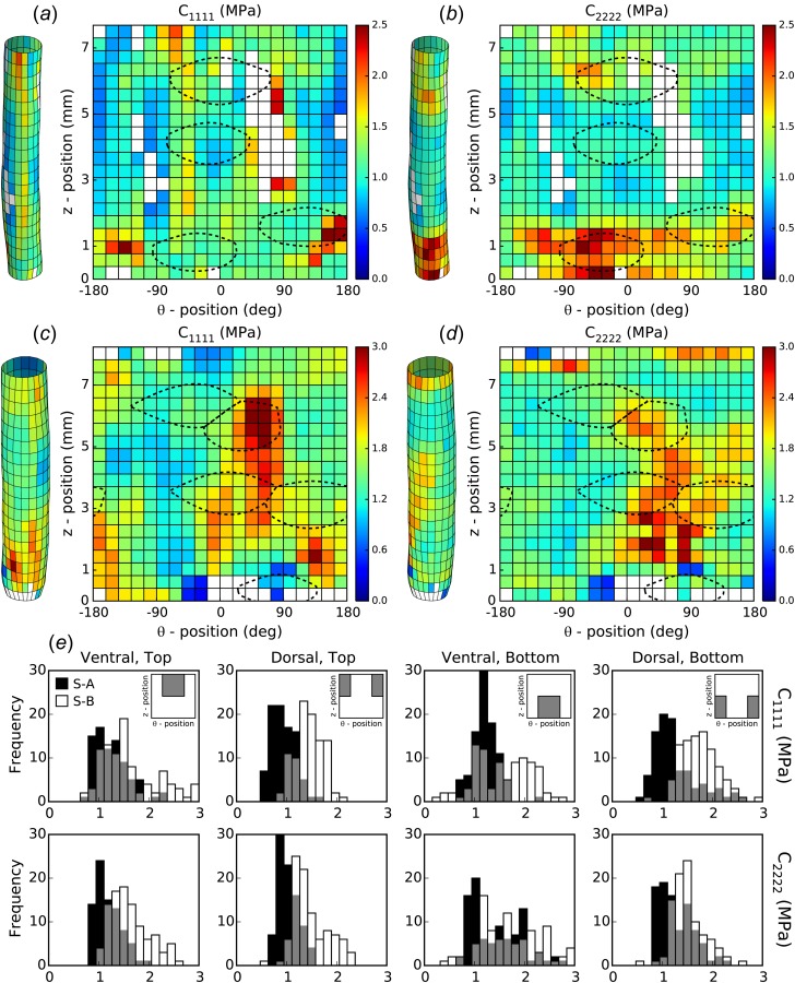
Spatial distribution of biaxial material stiffness. The biaxial material stiffness was computed using the identified material parameters over the surface of ((a) and (b)) sample A and ((c) and (d)) sample B. The results are shown for ((a) and (c)) circumferential (${\mathrm{C}}_{1111}$) and ((b) and (d)) axial (${\mathrm{C}}_{2222}$) stiffness evaluated at a loaded configuration of P(t) = 100 mmHg and λ_z(t) = λ⁰. Regions of influence due to branches (dashed lines) are overlaid to show localization near regions of high stiffness. (e) Histograms show spatial distributions in each quadrant for both samples (cf. Fig. 3).