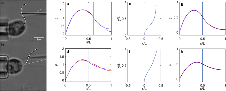
Figure 5.
Examples of analytical solutions fitted to counterbend data from (a–d) experiment and (e–h) simulation. (a) Flagellum of wild-type Chlamydomonas (Fig. 3, a and c) with manually picked points (black dots) and a polynomial curve (thick white line) fitted to these points. The flagellum before bending is also shown (thin white line). (b) Flagellum of pf3; cnk11-6 Chlamydomonas (Fig. 3, b and d) with manually picked points (black dots) and a polynomial curve (white) fitted to these points. (c) Values of θ(s) (red dots) from polynomial curve fit in (a), and fitted solution (blue curve; Eqs. 12a and 12b) with β2 = 0.202, (βL)2 = 25.5. (d) Values of θ(s) (red dots) from a polynomial curve fit in (b), and a fitted solution (blue curve; Eqs. 12a and 12b) with β2 = 0.053, (βL)2 = 5.0. (e) Simulated shape of a beam with (βL)2 = 25. (f) Simulated shape of a beam with (βL)2 = 5. (g) Values of θ(s) at 50 equally spaced points on flagellum (red dots) from simulation with (βL)2 = 25 and fitted solution (blue curve; Eqs. 12a and 12b). (h) Values of θ(s) (red dots) from simulation with (βL)2 = 5 and fitted solution (blue curve; Eqs. 12a and 12b). To see this figure in color, go online.

