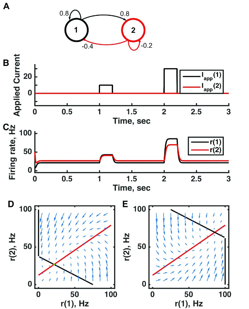
Figure 1. A single point attractor is present without input and a different one with input in a threshold-linear two-unit circuit.

( A) Diagram of the model circuit. Arrows indicate excitatory connections, and balls indicate inhibitory connections between units. ( B) Applied current as a function of time. Two different sized pulses of current are applied to unit 1. ( C) Firing rate as a function of time in the coupled network. During each current step, a new attractor is produced, but following current offset the original activity state is reached. ( D) Any particular combination of the firing rates of the two units (x-axis is rate of unit 1, y-axis is rate of unit 2) determines the way those firing rates change in time (arrows). Starting from any pair of firing rates, any trajectory following arrows terminates at the point of intersection of the two lines. Red line: nullcline for unit 2—the value of r(2) at which dr(2)/dt = 0 (its fixed point) given a value of r(1). Since unit 1 excites unit 2, the fixed point for r(2) increases with r(1). Black line: nullcline for unit 1—the value of r(1) at which dr(1)/dt = 0 (its fixed point) given a value of r(2). Since unit 2 inhibits neuron 1, the fixed point for r(1) decreases with r(2). The crossing point of the nullclines is a fixed point of the whole system. The fixed point is stable (so is an attractor state) because arrows converge on the fixed point. ( E) As in (D) but the solution during the second pulse of applied current. The applied current shifts the nullcline for r(1) so that the fixed point of the system is at much higher values of r(1) and r(2). For parameters, see supporting Matlab code, “dynamics_two_units.m”.