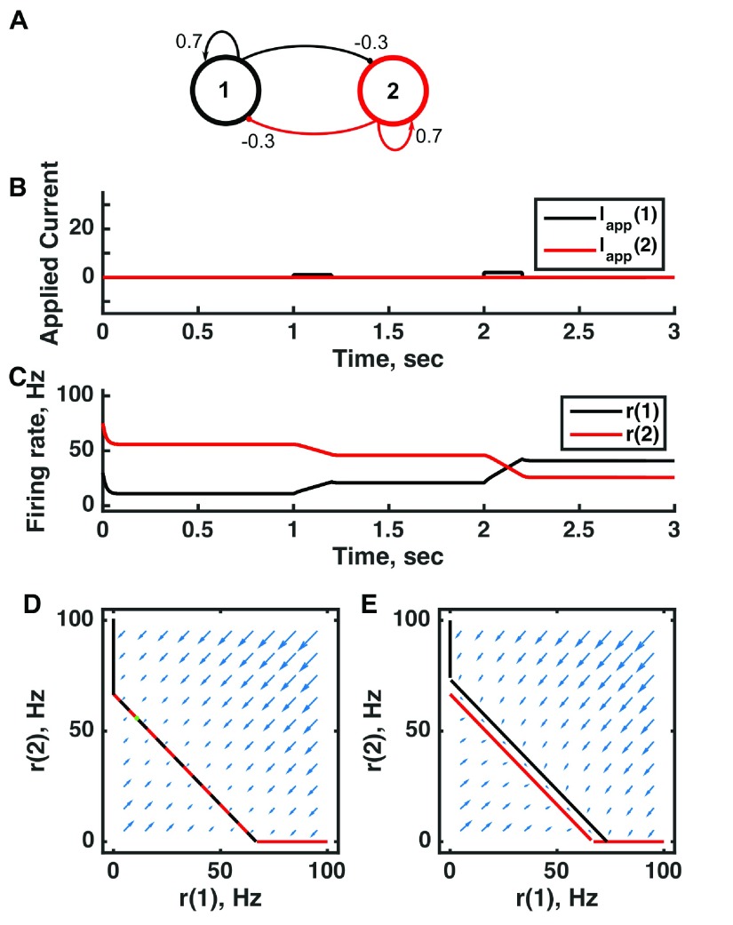
Figure 5. A marginal state or continuous/line attractor is produced by careful tuning of the connection strengths in a threshold-linear two-unit circuit.

( A) Diagram of the model circuit. Arrows indicate excitatory connections, and balls indicate inhibitory connections between units. The architecture is identical to that of Figure 2. ( B) Applied current as a function of time. Two very small pulses of current are applied to unit 1. ( C) Firing rate as a function of time in the coupled network. During each current step, the firing rate of unit 1 increases linearly because of the applied current. Inhibitory feedback to unit 2 causes a linear decrease in its firing rate. Upon stimulus offset, the firing rate reached is maintained. ( D) Any particular combination of the firing rates of the two units (x-axis is rate of unit 1, y-axis is rate of unit 2) determines the way those firing rates change in time (arrows). Starting from any pair of firing rates, any trajectory following arrows terminates at a point where the two lines overlap each other. Red line: nullcline for unit 2—the value of r(2) at which dr(2)/dt = 0 (its fixed point) given a value of r(1). Black line: nullcline for unit 1—the value of r(1) at which dr(1)/dt = 0 (its fixed point) given a value of r(2). Since the two units inhibit each other, the overlapping lines have negative gradient. ( E) A small applied current to unit 1 shifts its nullcline to the right slightly. Now the only fixed point is where the two lines intersect at r(2) = 0, but in the region between the two parallel nullclines, the rate of change is small (note the small arrows parallel to the lines) so firing rates change gradually. For parameters, see supporting Matlab code, “dynamics_two_units.m”.