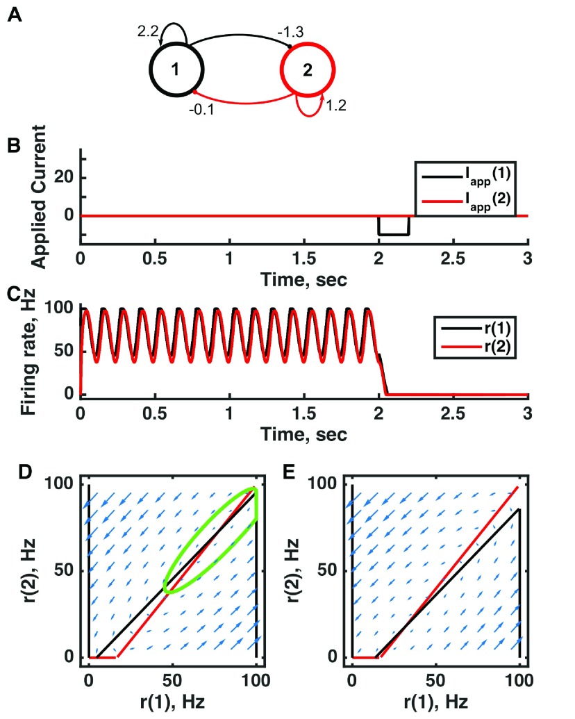
Figure 6. An oscillator produced by directed excitatory and inhibitory connections in a bistable threshold-linear two-unit circuit.

( A) Diagram of the model circuit. Arrows indicate excitatory connections, and balls indicate inhibitory connections between units. The architecture is identical to that of Figure 1 and Figure 3. ( B) Applied current as a function of time. An inhibitory pulse of current is applied to unit 1. ( C) Firing rate as a function of time in the coupled network. Oscillations are switched off by the inhibition to unit 1, so the system has two stable attractors: one a limit cycle, the other a point attractor. ( D) Any particular combination of the firing rates of the two units (x-axis is rate of unit 1, y-axis is rate of unit 2) determines the way those firing rates change in time (arrows). Depending on the starting point, a trajectory following the arrows will fall on the limit cycle (the green closed orbit, which represents the coordinated variation of firing rate with time during the oscillations) or will reach the fixed point at the origin. Red line: nullcline for unit 2—the value of r(2) at which dr(2)/dt = 0 (its fixed point) given a value of r(1). Since unit 1 excites unit 2, the fixed point for r(2) increases with r(1). Black line: nullcline for unit 1—the value of r(1) at which dr(1)/dt = 0 (its fixed point) given a value of r(2). Crossing points of the nullclines are the fixed points of the whole system, but the one within the limit cycle is unstable, as is the one with r(2) = 0 but r(1) > 0. ( E) As in ( D) but the solution during the inhibitory pulse of applied current. The inhibitory current shifts the nullcline for r(1) down, and the result is that all trajectories terminate at the origin. For parameters, see supporting Matlab code, “dynamics_two_units.m”.