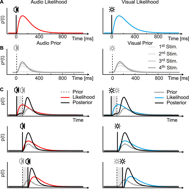
Figure 5. Bayesian model of perceived stimulus timing with asymmetric probability distributions (see Methods for details).

(A) The top panel shows the likelihood probability distribution – the probability of sensing the stimulus presented at t = 0. The distribution is obtained by through an exponential low pass filtering of the input signal⁶⁶. (B) The prior probability distribution for the next stimulus is obtained by combining the prior for the previous stimulus with the current posterior distribution, plus a constant (Methods, Equation 7). (C) Integration of prior and likelihood to obtain the posterior distribution according to Equation 6 for the fourth stimulus (last stimulus in Experiment 2) appearing −40 ms, 0 ms, or +40 ms with respect to the expected time (separate rows). Perceived timing is obtained retrospectively by considering the overall posterior distribution (i.e., by computing the mean of the distribution).