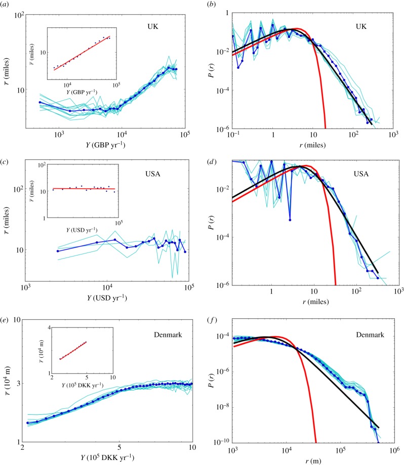
Figure 1.

(a,c,e) Average commuting distance versus income for different years. In dark blue, the commuting distance is averaged over all years. (a) UK data. This log–log plot displays a plateau for small values of income followed by a regime, when fitted by a power law (see inset), gives an exponent β ≈ 0.5 ([0.53,0.66]). In the inset, the average commuting distance is averaged over all years, and the power law fit gives an exponent β ≈ 0.58. (c) US data. In this log–log plot, we do not observe an income dependence. Indeed, a power law fit gives an exponent β ≈ 0. (e) Danish data. The power law fit on the commuting distance averaged over all years (in the inset) gives an exponent β ≈ 0.77. (b,d,f) Commuting distance distribution for different income classes. The probability distribution is shown for different income classes. In dark blue, we show the distribution for a particular value of the income for which fits have been performed. In red, we show the one parameter fit with the analytical function predicted by the extended McCall model (equation (3.8)), and in blue, the one parameter fit with the analytical function predicted by the closest opportunity model (equation (3.15)). (b) UK data (averaged over all available years). (d) US data (averaged over all available years). (f) Danish data (all years give the same result and we choose here to show the year 2008). In all cases, we observe that the tail predicted by the extended McCall model (equation (3.8)) decays too quickly and cannot fit the data for long distances. In contrast, the closest opportunity model is in excellent agreement with empirical observations. (Online version in colour.)