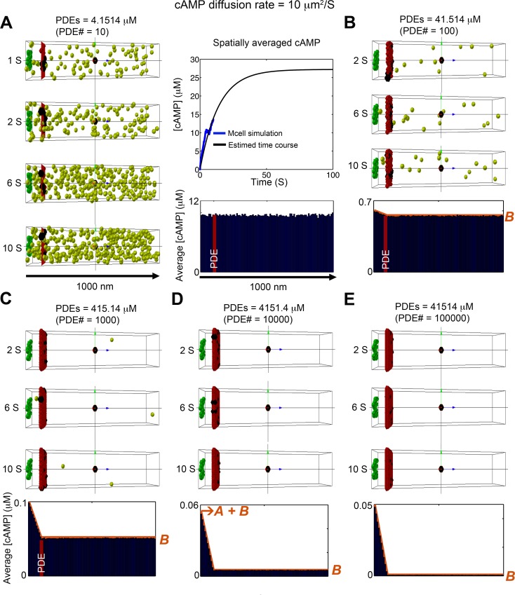
Fig 4. Stochastic simulation of cAMP diffusion implemented in MCell and visualized using CellBlender.

The diffusion coefficient was set to 10 μm²/s. (A) 10 PDE molecules (~4.1514 μM). Four snapshots are shown in the left, the average cAMP concentration for the 1800 time frames between 1s to 10s are shown shown in the blue bar graph, and the time course of the spatially averaged cAMP concentration is shown in the top right panel. (B) PDE molecules = 100 (~41.514 μM). Average of cAMP molecules for 1800 time frames from 1s to 10s at steady state. (C) PDE molecules = 1000 (~415.14 μM). Average of cAMP molecules over 1800 time frames from 1s to 10s at steady state. (D) PDE molecules = 10000 (~4151.4 μM). Average of cAMP molecules for 1800 time frames from 1s to 10s at steady state. (E) PDE molecules = 100000 (~41514 μM). Average of cAMP molecules over 1800 time frames from 1s to 10s at steady state. The red curves plotted on the accumulated concentration maps in panel (B-E) show the predictions of the 1D continuum model. In all cases, there is excellent agreement with the full 3D stochastic model. The cAMP compartmentation ratio R for the various values of PDE concentration shown in panels (A-E) are 1.826 x 10⁻³, 8.381 x 10⁻², 4.970 x 10⁻¹, 9.087 x 10⁻¹, and 9.901 x 10⁻¹,