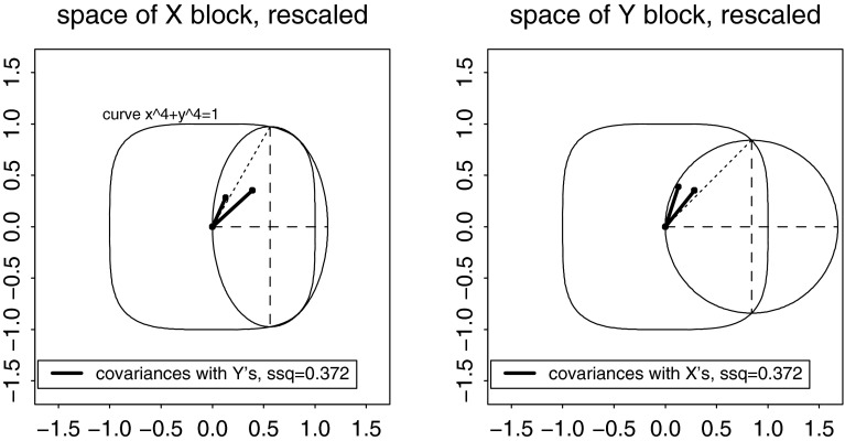
Fig. 11.

Geometry of the RV coefficient for two blocks of two measures each. The rounded square in each frame is the curve $x^4+y^4=1$ that normalizes the trace of the square of either $2\times 2$ covariance matrix. Each ellipse is aligned with its axes horizontal and vertical and the end of the shorter axis running through the center (0, 0) of the quartic curve. Then each is scaled so that its “diagonal”—the vector from the end of one axis to the end of the other—lies upon the quartic. With this joint scaling, the RV coefficient is the sum of the squared lengths of the heavy vectors out of (0, 0) in either figure: the vectors representing either the rows (left) or the columns (right) of the normalized covariance matrix $z_X{z}_Y{s}_{P{C}_{Xi}P{C}_{Yj}}$. The text argues that this computation is without biological meaning