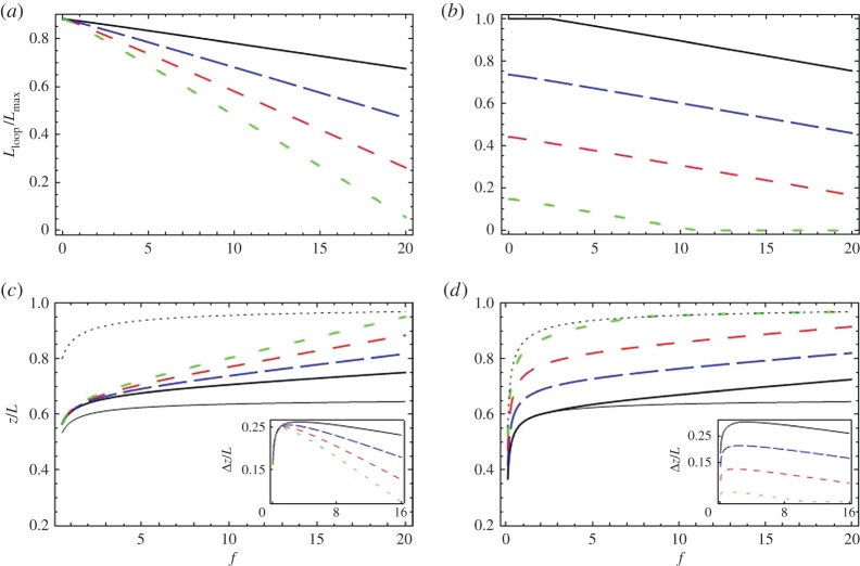
Figure 3.

Exploring the effects predicted by model 2. We show, as in figure 2, plots of L_loop and z for various values of model parameters, calculated using equations (3.1), (3.2) and (3.5). Again, a value of l_p=500 Å is used (in equation (3.2)). Plots of L_loop, normalized over $L_{max}\approx 34\hspace{0.17em}000$ Å (the maximum length for pairing of the homologous segments), are shown in (a,b). Plots of z divided by the total DNA length L are shown in (c) and (d). As in figure 2, the thin solid line is the extension-force curve expected for total homologous pairing ($L_{\mathrm{loop}}=L_{max}$) and the thin dotted line is that for no pairing (L_loop= 0). The insets in (c,d) show Δz—the difference in extension curves with no pairing at all (thin dotted line) and those generated with homologous pairing. In (a,c), L₀=30 000 Å and the thick solid, long dashed, medium dashed and short dashed lines correspond to the values of β=15 000, 30 000, 45 000, 60 000 Ų/k_BT. In (b,d), β= 20 000 Ų/k_BT and the solid, long dashed, medium dashed and short dashed lines correspond to the values L₀=35 000, 25 000, 15 000, 5000 Å(we considered even one value of L₀ larger than $L_{max}$ but, as L_loop can never exceed $L_{max}$, in (b) the magnitude of L_loop is limited to $L_{max})$. (Online version in colour.)