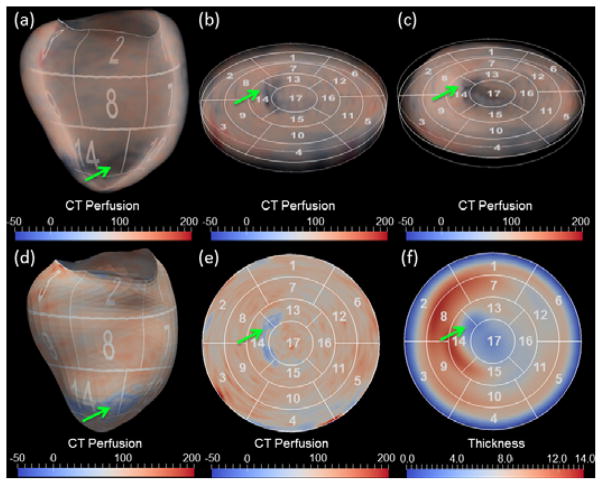
Fig. 4.
LV visualization using 3D volume rendering (top row) and 2D surface rendering (bottom row). In both cases, the LV is flattened from 3D (a, d) to 2D thick (b, c) or thin (e, f) slices in order to display the LV on the polar map. CT perfusion was rendered with uniform and absolute thickness in (b) and (c), respectively. The aggregated perfusion and thickness are shown in the (e) and (f), respectively. The green arrows point to the perfusion and myocardial thickness abnormalities.

