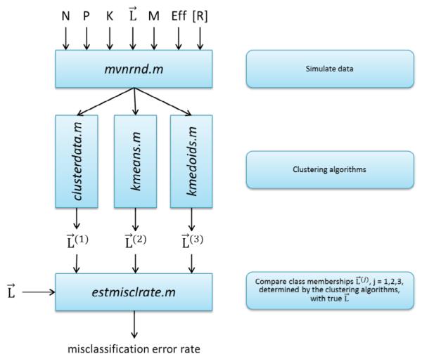
Figure 1.

Schematic representation of the analysis. Analysis involves three parts. First, simulate data based on the following inputs: P-number of patients, N-number of proteins in the assay, K- number of patient clusters, L –list of class membership with P elements, where each element Li (i=1,2,…P) is an integer q=1,2,…K. Other inputs are: M – number of differentially abundant proteins (candidate biomarkers), Eff_nq- effect size (could be different for each protein n and each cluster q), R- correlation matrix of protein abundances. Second, use simulated data as an input to the clustering algorithms (in this paper: hierarchical clustering, k-means, and k-medoids). Third, compare lists of class memberships L^(r) r=1,2,3 generated by the clustering algorithms with the true list of class membership L; determine misclassification error rate. Vary inputs, e.g. Eff and P, repeat the whole procedure, create plots of misclassification error vs. Eff. Determine the threshold value of effect size which enables misclassification error below 5% for the given number of patients P, or determine the number of patients (sample size of the future study), which enables misclassification error below 5% for the given expected Eff. See detailed explanation in the text.