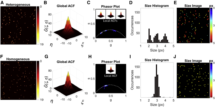
Figure 2.
Analysis of polydisperse (A–E) and monodisperse (F–J) randomly distributed Gaussians with SNR = 10. The monodisperse sample consists of 100 elements with FWHM = 3 px, whereas the polydisperse sample consists of 33 elements with FWHM = 2 px, 33 with FWHM = 3 px and 34 with FWHM = 4 px. (B and G) Global ACFs computed on the intensity images (A) and (F), respectively. (C and H) Phasor plots of (A) and (F) compared with the m = 10 calibration curve (white dashed line), with examples of local ACFs shown in the insets. (D and I) Size histograms obtained from the size images (E and J) of (A) and (F), respectively. To see this figure in color, go online.

