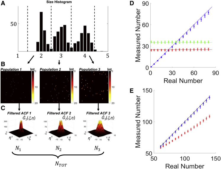
Figure 4.
(A) Size histogram of a polydisperse sample of particles, SNR = 10, where the black dotted lines visually show the segmentation performed (1.5 px < size1 < 2.5 px, 2.5 px < size2 < 3.5 px, 3.5 px < size3 < 4.5 px) to obtain the segmented images in (B), shown from the smaller (population 1) to the larger (population 3). (C) Filtered ACFs corresponding to the segmented populations, from which the number of elements of each population has been retrieved (N1, N2, and N3). (D) Retrieved number of a single population (circles) shown as the mean value of a set of 100 realizations, the error bar being the standard deviation; populations 1–3 correspond to blue, red, and green circles, respectively, and the dash-dotted lines show the actual number for each population; populations 2 and 3 were simulated with a constant number (25 and 35, respectively), whereas the population 1 number was varied from 1 to 80. (E) Retrieved total number (blue circles) compared with traditional ICS analysis (red circles) of the same samples in (D). To see this figure in color, go online.

